Understanding the Normal Distribution Curve

In This Article

1. What Is the Normal Distribution Curve?

2. Normal Distribution Key Terms

3. The Importance of the Normal Distribution Curve

4. Normal Distribution Notation and Formula

5. The Empirical Rule

6. Standard Normal Distributions

7. How To Interpret a Normal Distribution Curve

In 1733, a French mathematician named Abraham de Moivre was working a side hustle as an advisor to gamblers and insurance agents. For his gambler clients, de Moivre was looking for a shortcut to calculate the probability of winning money from a repeated game like a coin flip. De Moivre discovered that a smooth and symmetric bell-shaped curve with a precise formula could approximate the winnings—if played enough times.

Nearly 80 years later, Carl Friedrich Gauss—the famous German mathematician and physicist—popularized this distribution, now known as the Gaussian or normal distribution. The normal distribution is central in statistics. We can apply it to many real-world phenomena, not just probabilities for gamblers!

What Is the Normal Distribution Curve?

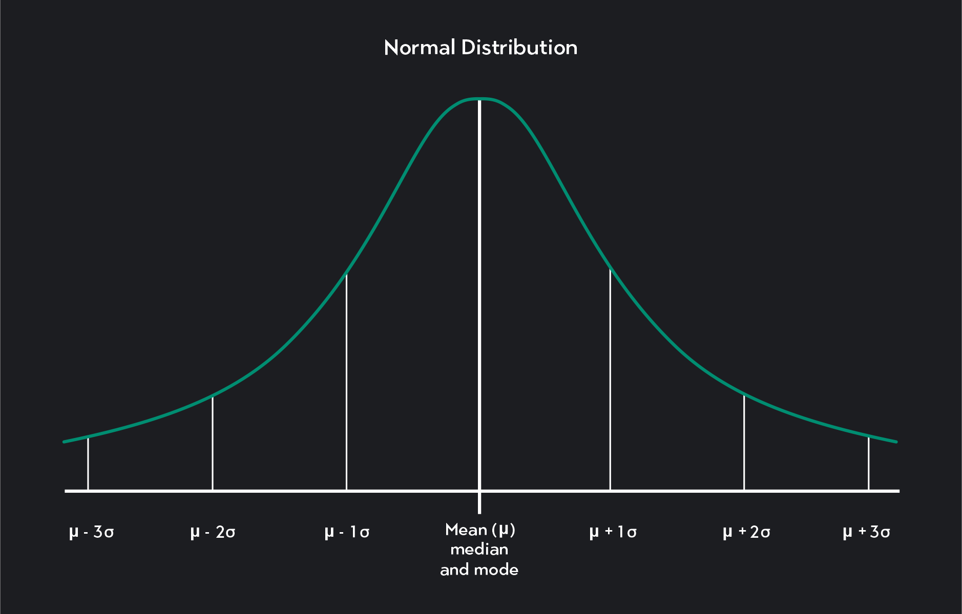
A normal distribution—also known as a bell curve, Gaussian distribution, or Gauss distribution—is a continuous probability distribution that is bell-shaped and symmetric around the mean. It is the most widely used probability distribution in statistics. A normal distribution curve is a graph or visual representation of the normal distribution.

One of Outlier’s instructors, Dr. Olanrewaju Michael Akande of Duke University, gives an over of normal distribution:

Normal Distribution Key Terms

Probability Distributions

A probability distribution is a function that gives you the probability or likelihood of observing a particular value (or a subset of values) of a random variable. We often represent graphically probability distributions to provide a visual representation of the distribution. Other well-known probability distributions include:

• The uniform distribution

• The binomial distribution

• The Poisson distribution

• The Student’s t distribution

• The Chi-squared distribution

• The exponential distribution

Discrete and Continuous Probability Distributions

Probability distributions can be discrete or continuous.

Discrete probability distributions are probability distributions for discrete random variables. Discrete random variables are random variables that take on distinct and countable values. Continuous probability distributions are probability distributions for continuous random variables—i.e., random variables that can take on an infinite number of values within a given range. Continuous probability distributions take two primary forms: probability density functions (PDFs) and cumulative distribution functions (CDFs).

Mean, Median and Mode of a Distribution

Mean, median, and mode are all measures of center.

The mean is the average value of the distribution.

The median divides the distribution in half with 50% of the observations above the median and 50% below the median.

The mode is the most frequently occurring value in the distribution. Because we measure mean, median, and mode differently, they are usually not equal. A key feature of a normally distributed variable is that its mean, median, and mode are all the same.

Skewness and Symmetry

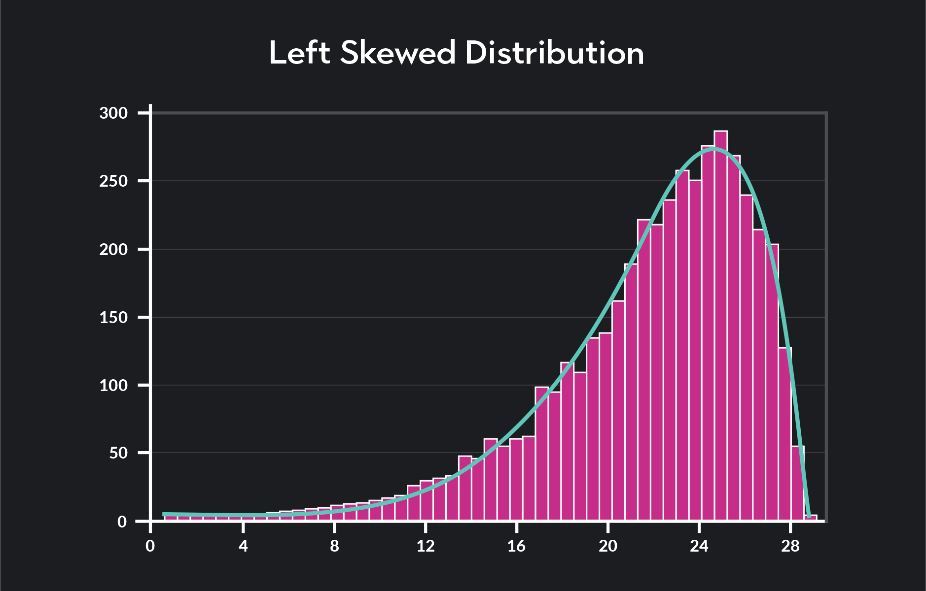
Skewness measures how asymmetrical a distribution is relative to its mean. If a distribution has a tail that trails off to the left, we say that the distribution has a negative or left skew.

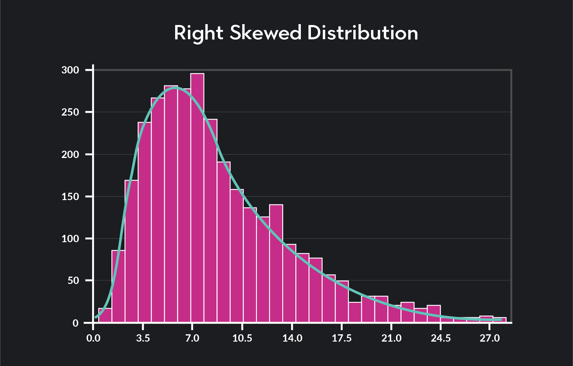
If a tail trails off to the right, we say that the distribution has a positive or right skew.

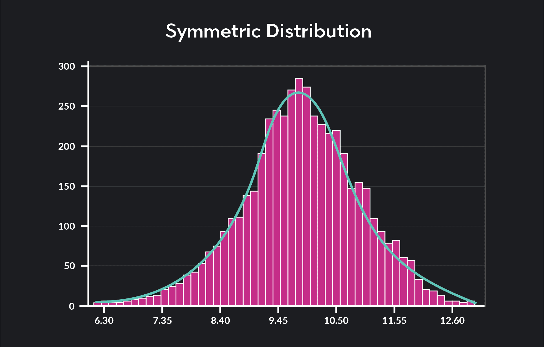
A distribution with no skewness is symmetric around the mean, meaning the part of the distribution. To the right of the mean will be the exact mirror image of the part of the distribution that lies to the left of the mean. Normal distributions are symmetric.

The Standard Deviation of a Distribution

Standard deviation is a measure of spread. It tells you how much variation there is in the data relative to the mean. A distribution—where all the data points are closely clustered around the mean—will have a low standard deviation. Data that is widely dispersed around the mean will have a high standard deviation.

The Importance of the Normal Distribution Curve

Normal distributions play a major role in statistical analysis for three main reasons.

1. Approximation

First, a normal distribution can approximate many things we observe in life. Some examples of random variables that a normal distribution can approximate are:

• Standardized test scores

• The heights and weights of people

• Blood pressure

• Errors in measurement

2. Sampling Distribution

Second, the Central Limit Theorem tells us that if certain conditions are met, the sampling distribution of the sample mean $\bar{x}$ will also be normally distributed. This idea is central to a lot of statistical inferences we make about populations using sample data sets.

3. An Easy Process

Third, calculating probabilities for normally distributed variables—or variables that are approximately normal—is a quick and easy process. By knowing two things about a normally distributed variable—the mean $\mu$ and the standard deviation $\sigma$—you can use the empirical rule and Z-score transformations to make all kinds of statistical inferences about the variable.

Characteristics of Normal Distributions

The main characteristics of a normal distribution are:

Unimodal

It is unimodal, meaning it has one mode.

Bell-shaped

It is bell-shaped with most of the observations lying within one standard deviation of the mean and nearly all observations lying within three standard deviations of the mean.

Symmetric

It is symmetric. The portion of the distribution that lies to the left of the mean is the mirror image of the portion of the distribution that lies to the right of the mean. Another way of saying this is that the distribution does not skew to the left or the right (the skewness of the distribution = 0).

Mean = Median = Mode

The mean, median, and mode are all equal (mean = median = mode). This means that exactly half of the observations in a normal distribution fall below the mean, and half of the observations are above the mean.

Shape Controlled by Mean and Standard Deviation

The mean and standard deviation of the random variable controls the exact shape of a particular normal distribution. The mean $\mu$ tells you where the distribution is centered, and the standard deviation $\sigma$ tells you how wide or narrow the distribution is.

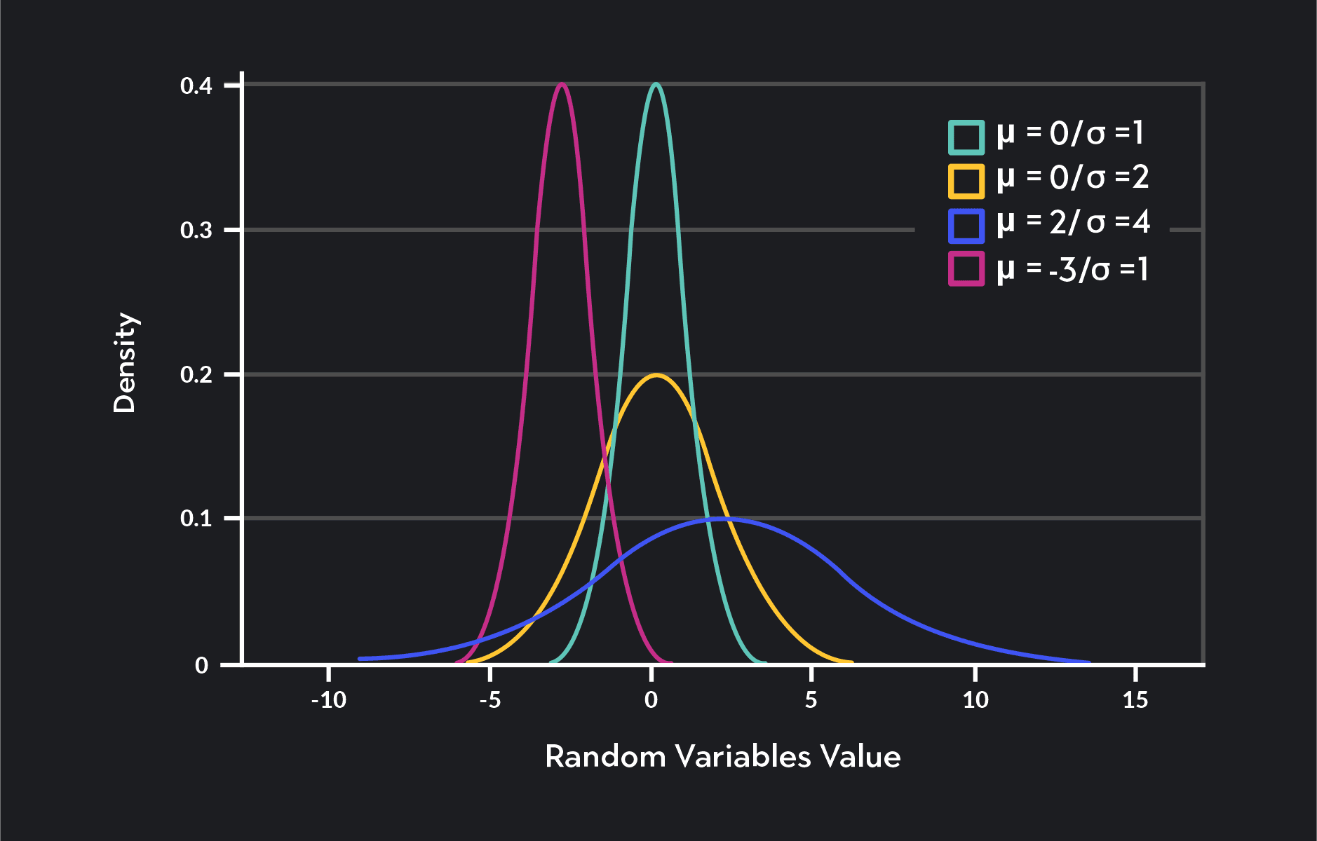
Examples of some normal distributions

Normal Distribution Notation and Formula

You might see the following notation used to indicate that a random variable, X, is normally distributed:

X is the random variable that is normally distributed with a mean $\mu$ and a standard deviation $\sigma$

The probability density function (PDF) of a normal distribution takes the form:

The Empirical Rule

The empirical rule—also known as the 68-95-99.7 rule—highlights three basic probabilities related to the normal distribution. We can apply it to any normal distribution regardless of the mean or standard deviation of the distribution.

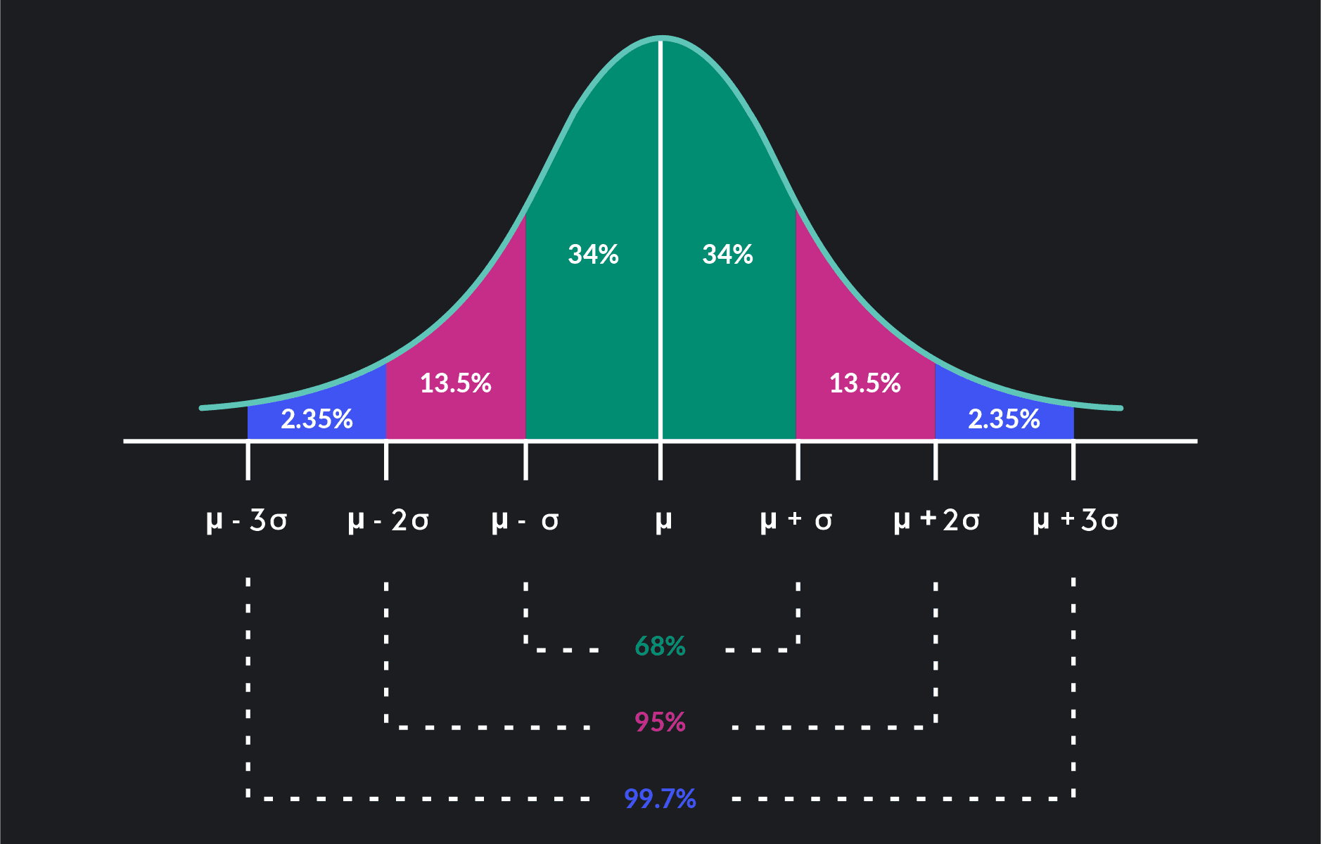
The Empirical Rule (68-95-99.7 Rule)

The empirical rule states that in a normal distribution:

• 68 percent of all observations lie within one standard deviation of the mean

• 95 percent of all observations lie within two standard deviations of the mean

• 99.7 percent of all observations lie within three standard deviations of the mean

Notice that from these probabilities, you can calculate numerous others.

For example, we can say that 34% of the observations are within one standard deviation to the right of the mean. Then 34% of the observations are within one standard deviation to the left of the mean. Because (100-99.7)÷2 = 0.15, we can say that only 0.15% of all observations are beyond three standard deviations to the right of the mean.

Almost all observations in a normal distribution—99.7 percent of them—lie within three standard deviations of the mean. Statisticians sometimes refer to the empirical rule as the three-sigma rule of thumb or the 3 sigma rule.

Standard Normal Distributions

A standard normal distribution—also known as a Z-distribution—is a normal distribution with a mean equal to zero ($\mu$=0) and a standard deviation equal to 1 ($\sigma$=1).

The standard normal distribution is a special case of the normal distribution. The letter Z often denotes it rather than the letter X. Any particular value of Z is called a Z-score or standard score.

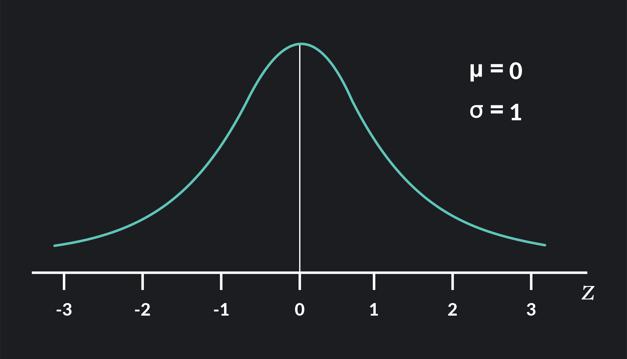
Although very few things in the world have a standard normal distribution, it plays a crucial role in statistics. It provides a shortcut for calculating probabilities for non-standard normal distributions through a process called standardization or Z-transformations.

In a Z-transformation, we map values from a normal distribution to a particular Z-score in the standard normal distribution. You can always map a value from a normal distribution to a particular Z-score.

The advantage of doing this is that we associate all Z-scores with precise probabilities that you can look up. We can see them in statistical tables called “standard normal distribution tables'' or by using statistical software such as R, Desmos, and Stata. By performing Z-transformations, you can easily look up probabilities for normal distributions instead of performing complicated calculations.

In the next section, we provide an example of how to do this.

The formula for Z-transformations is:

How To Interpret a Normal Distribution Curve

Below is a graph of a normal distribution. In this example, the random variable, X, represents the height of adult women in the United States. A normal distribution can approximate X and has a mean equal to 64 inches (about 5ft 4in), and a standard deviation equal to 2.5 inches ($\mu$=64 in, $\sigma$ =2.5 in).

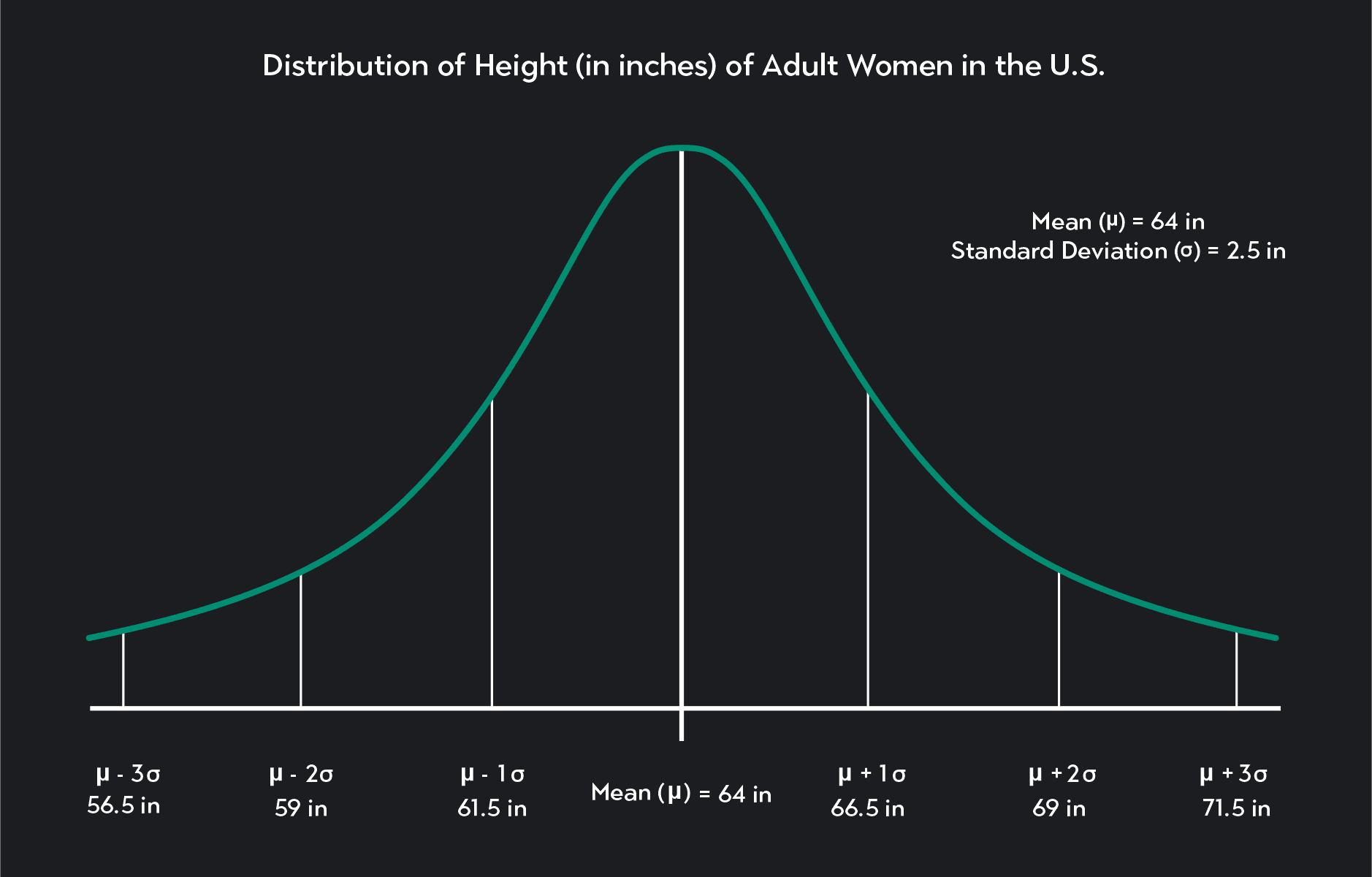
• $X$ is the height of adult women in the United States

• $\mu$ is the mean height and is equal to 64 inches

• $\sigma$ is the standard deviation and is equal to 2.5 inches

Let’s take a step-by-step look at how to interpret this graph and how to apply both the empirical rule and Z-transformations to calculate some probabilities.

1. Finding Probabilities

In a continuous probability distribution—like a normal distribution—there are an infinite number of possible values that the random variable X can take. For this reason, the probability that X will be equal to any ‌value is equal to zero Pr(X=x) = 0.

When working with continuous probability distributions, the probabilities we are interested in are not the probabilities that X=x.

Instead, the probabilities are:

• X will be less than or equal to some value Pr (x≤a)

• X will be greater than or equal to some value Pr (x≥b)

• X falls within a specified range Pr (a ≤ x ≤ b)

In this example, the probability that an American woman is exactly 65.02301 inches tall is zero.

We could use the distribution to calculate the probability that an American woman is:

• Less or equal to 5ft (60 inches) tall

• Taller than 5ft7 inches (67 inches)

• Between 61.5 inches and 66.5 inches

Specific values on the bell curve do not represent these probabilities. The areas underneath the bell curve represent them, as shown in the figures below.

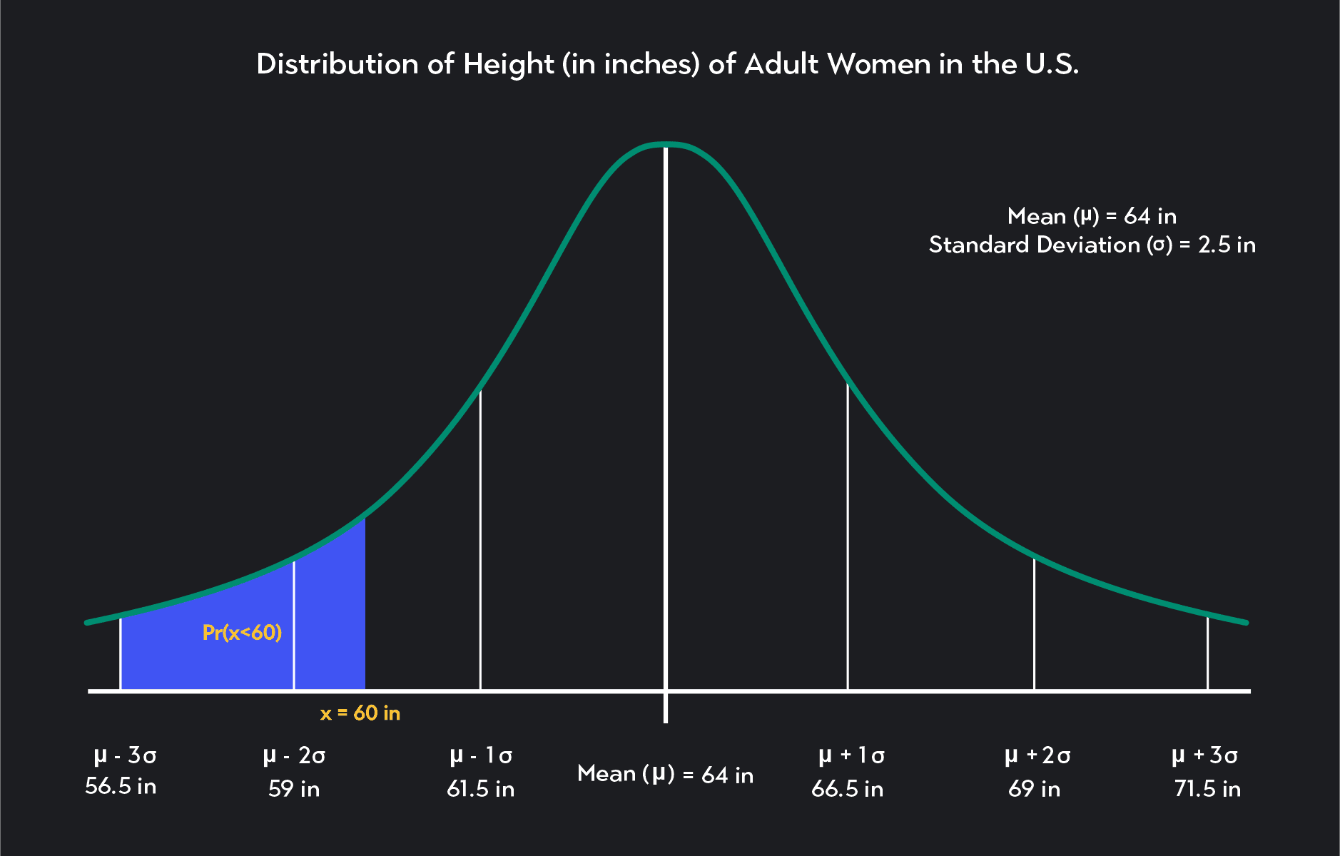
The probability that an American woman will be less than 60 inches tall

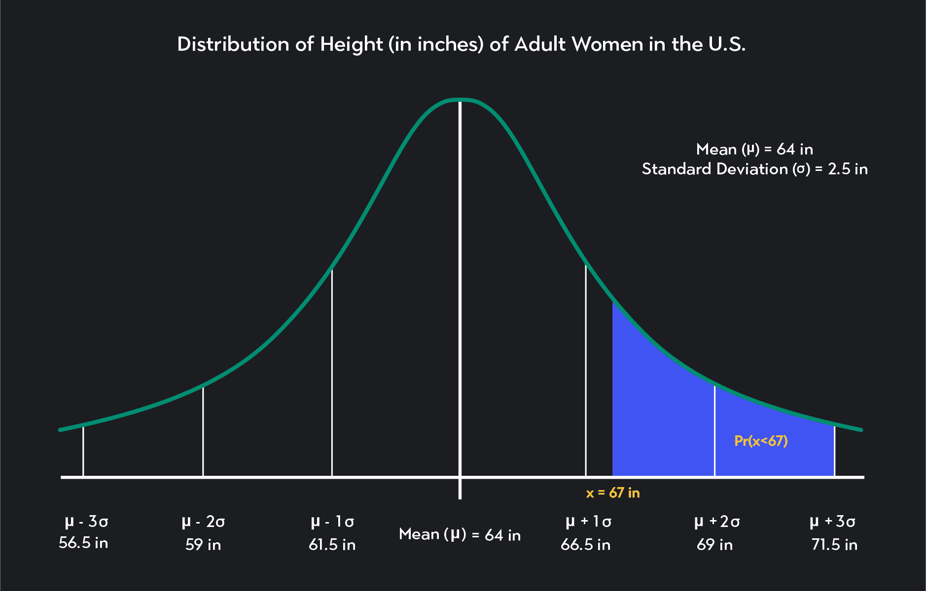
The probability that an American woman will be more than 67 inches tall

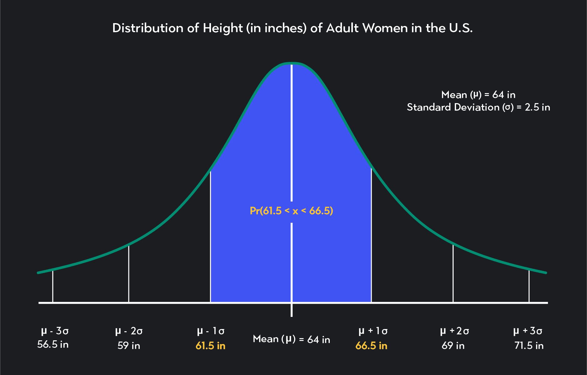
The probability that an American woman will be between 61.5 and 66.5 inches tall

2. Using the Empirical Rule

To calculate the probabilities we want, we could use integrals to calculate the total area under the curve within our specified values. But, as we already discussed, there’s a shortcut. We can make use of the empirical rule or Z-transformations. Let’s start with the empirical rule and see if we can answer a few questions.

The Empirical Rule (68-95-99.7 Rule)

Question 1

What is the probability that an American woman is between 61.5 inches and 66.5 inches tall? What is Pr(61.5 ≤ x ≤ 66.5)?

To answer this question, think about how we represent these heights in terms of the mean and standard deviation.

Notice that 61.5 inches is equal to the mean minus one standard deviation.

Similarly, 66.5 inches is equal to the mean plus one standard deviation.

Solving the problem is now easy! The probability Pr(61.5 ≤ x ≤ 66.5) is the same as the probability that X is within one standard deviation of the mean. From the empirical rule, we know ‌the answer is 68%.

Question 2

What is the probability that an American woman is 59 inches tall (4ft 11 in) or shorter? What is Pr(x≤59 in)?

Again, notice that 59 inches are equal to the mean minus two standard deviations: $\mu$-2$\sigma$ = 64 - (2)(2.5) = 59 inches.

Looking at the graph for the empirical rule, see if you can now calculate the probability we are looking for: Pr(x≤59).

The answer is 2.5%. So 59 inches are two standard deviations below the mean. Because we want to know the likelihood that a woman is less than or equal to 59 inches tall, we are looking for the probability that x lies to the left of $\mu$-2$\sigma$.

We know that 50% of the distribution lies to the right of the mean, and an additional 47.5% (34% + 13%) of observations lie between the mean and the mean minus two standard deviations.

If we subtract these figures from 100%, we get the probability of observations that lie to the left of $\mu$-2$\sigma$.

3. Using Z-transformations

The empirical rule is handy for calculating probabilities involving values that are a fixed number of standard deviations from the mean—0, 1, 2, or 3 standard deviations from the mean. But it is less handy when we want to calculate probabilities that involve values that are 1.2 or 2.35 standard deviations from the mean.

To solve these types of probabilities, we can use Z-transformations.

Question 3

What is the probability that an American woman is shorter than 67 inches tall? What is Pr(x<67 in)?

The first step in solving a question like this is to find a Z-score using a Z-transformation. Recall that to find the Z-score, you have to subtract the mean, 𝜇, from the observed value, x, and then divide the difference by the standard deviation, σ.

If we follow the Z-score formula, we find that the Z-score associated with a height of 67 inches is 1.2. This Z-score tells us that the value of 67 inches is 1.2 standard deviations above the mean in our original normal distribution. The value of 67 inches maps to a Z-score of 1.2 because 1.2 is 1.2 standard deviations above the mean in a standard normal distribution.

The probability in this question is the percentage of women who are shorter than 67 inches. So we need to find the probability that Z is less than 1.2 in a standard normal distribution (Pr (z<1.2)).

As we said earlier, we can look up probabilities associated with Z-scores using a standard normal table or statistical software. If you do this, you’ll find that the probability we are looking for is 86.9%—rounded to one decimal place. We can conclude that according to our data, 86.9% of American women are shorter than 5ft 7 inches.

We went over a lot about normal distribution. It is one of the most widely used probability distributions in statistics. Many people use it in various disciplines, including the social sciences and data science.

Explore Outlier's Award-Winning For-Credit Courses

Outlier (from the co-founder of MasterClass) has brought together some of the world's best instructors, game designers, and filmmakers to create the future of online college.

Check out these related courses:

Intro to Statistics

How data describes our world.

Explore course

Intro to Statistics

How data describes our world.

Explore course

Intro to Microeconomics

Why small choices have big impact.

Explore course

Intro to Microeconomics

Why small choices have big impact.

Explore course

Intro to Macroeconomics

How money moves our world.

Explore course

Intro to Macroeconomics

How money moves our world.

Explore course

Intro to Psychology

The science of the mind.

Explore course

Intro to Psychology

The science of the mind.

Explore course