Understanding Sampling Distributions: What Are They and How Do They Work?

In This Article

1. Overview

2. Why Are Sampling Distributions Important?

3. Types of Sampling Distributions: Means and Sums

Overview

A sampling distribution is the probability distribution of a sample statistic, such as a sample mean ($\bar{x}$) or a sample sum ($\Sigma_x$).

Here’s a quick example:

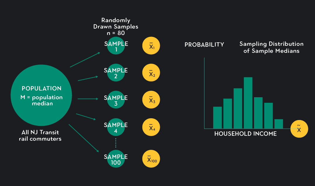
Imagine trying to estimate the mean income of commuters who take the New Jersey Transit rail system into New York City. More than one hundred thousand commuters take these trains each day, so there’s no way you can survey every rider. Instead, you draw a random sample of 80 commuters from this population and ask each person in the sample what their household income is. You find that the mean household income for the sample is $\bar{x}_{1}$ = $92,382. This figure is a sample statistic. It’s a number that summarizes your sample data, and you can use it to estimate the population parameter. In this case, the population parameter you are interested in is the mean income of all commuters who use the New Jersey Transit rail system to get to New York City.

Now that you’ve drawn one sample, say you draw 99 more. You now have 100 random samples of sample size n=80, and for each sample, you can calculate a sample mean. We’ll denote these means as $\bar{x}_1$, $\bar{x}_2$, … $\bar{x}_{100}$, where the subscript indicates the sample for which the mean was calculated. The value of these means will vary. For the first sample, we found a mean income of $92,382, but in another sample, the mean may be higher or lower depending on who gets sampled. In this way, the sample statistic $\bar{x}$ becomes its own random variable with its own probability distribution. Tallying the values of the sample means and plotting them on a relative frequency histogram gives you the sampling distribution of $\bar{x}$ (the sampling distribution of the sample mean).

Don’t get confused! The sampling distribution is not the same thing as the probability distribution for the underlying population or the probability distribution of any one of your samples.

In our New Jersey Transit example:

• The population distribution is the distribution of household income for all NJ Transit rail commuters. 

• The sample distribution is the distribution of income for a particular sample of eighty riders randomly drawn from the population.  

The sampling distribution is the distribution of the sample statistic $\bar{x}$. This is the distribution of the 100 sample means you got from drawing 100 samples.

Why Are Sampling Distributions Important?

Sampling distributions are closely linked to one of the most important tools in statistics: the central limit theorem. There is plenty to say about the central limit theorem, but in short, and for the sake of this article, it tells us two crucial things about properly drawn samples and the shape of sampling distributions:

1. If you draw a large enough random sample from a population, the distribution of the sample should resemble the distribution of the population. 

2. As the number of drawn samples gets larger and larger, and if certain conditions are met, the sampling distribution will approach a normal distribution.

What conditions need to be met for the central limit theorem to hold?

The central limit theorem applies in situations where the underlying data for the population is normally distributed or in cases where the size of the samples being drawn is greater than or equal to 30 (n≥30). In either case, samples need to be drawn randomly and with replacement.

Here is the magic behind sampling distributions and the central limit theorem. If we know that a sampling distribution is approximately normal, we can use the rules of probability (such as the empirical rule, z-transformations, and more) to make powerful statistical inferences. This is true even if the underlying distribution for the population is not normal or even if the shape of the underlying distribution is unknown. So long as the sample size is equal to or greater than 30, we can use the normal approximation of the sampling distribution to get a better estimate of what the underlying population is like.

A refresher on normal distributions and the empirical rule:

The normal distribution is a bell-shaped distribution that is symmetric around the mean and unimodal. 

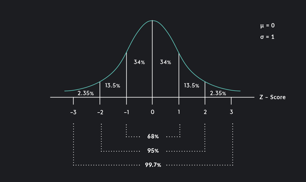
The empirical rule tells us that 68% of all observations in a normal distribution lie within one standard deviation of the mean, 95% of all observations lie within two standard deviations of the mean, and 99.7% of all observations lie within three standard deviations of the mean.

A refresher on standard normal distributions and z-transformations:

A standard normal distribution is a normal distribution with a mean equal to zero and a standard deviation equal to one. 

Any value from a normal distribution can be mapped to a value on the standard normal distribution using a z-transformation. 

$Z =\frac{(x-\mu)}{\sigma}$

Types of Sampling Distributions: Means and Sums

Sampling distributions can be constructed for any random-sample-based statistic, so there are many types of sampling distributions. We’ll end this article by briefly exploring the characteristics of two of the most commonly used sampling distributions: the sampling distribution of sample means and the sampling distribution of sample sums. Both of these sampling distributions approach a normal distribution with a particular mean and standard deviation. The standard deviation of a sampling distribution is called the standard error.

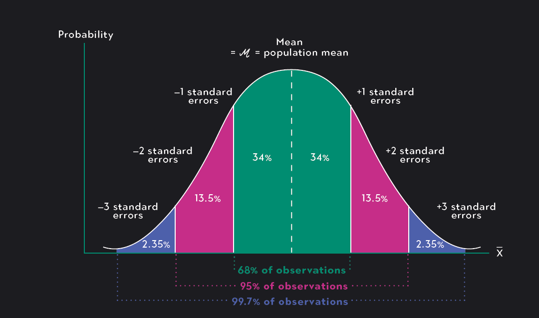
If the central limit theorem holds, the sampling distribution of sample means will approach a normal distribution with a mean equal to the population mean, $\mu$, and a standard error equal to the population standard deviation divided by the square root of the sample size, $\frac{\sigma}{\sqrt{n}}$.

The fact that the distribution of sample means is centered around the population mean is an important one. This means that the expectation of a sample mean is the true population mean, $\mu$, and using the empirical rule, we can assert that if large enough samples of size n are drawn with replacement, 99.7% of the sample means will fall within 3 standard errors of the population mean. Lastly, sampling distribution of means allows you to use z-transformations to make probability statements about the likelihood that a sample mean, $\bar{x}$, calculated from a sample of size n, will be between, greater than, or equal to some value(s).

The sampling distribution of sample means:

The sampling distribution of the sample means,  $\bar{x}$, approaches a normal distribution with mean,  $\mu$, and a standard deviation, $\frac{\sigma}{\sqrt{n}}$).

$\bar{x}$  ~ N($\mu$, $\frac{\sigma}{\sqrt{n}}$) where $\mu$ is the population mean, $\sigma$ is the population standard deviation, and n is the sample size

Just as the sampling distribution of sample means approaches a normal distribution with a unique mean and standard, so does the sampling distribution of sample sums. A sample sum, $\Sigma$, is just the sum of all values in a sample. 

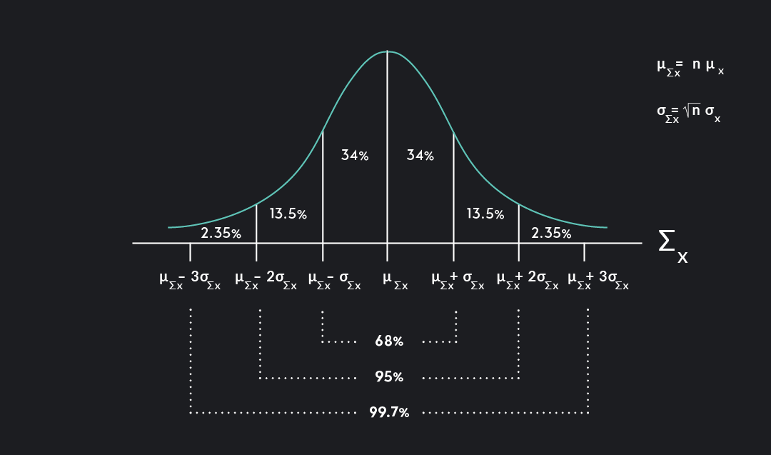
The sampling distribution of sample sums is centered around a mean equal to the sample size multiplied by the population mean, n$\mu$, and the standard error of sums is equal to the square root of the sample size multiplied by the standard deviation of the population: ($\sqrt{n}$)($\sigma$).

The sampling distribution of sample sums:

The sampling distribution of the sample sums, $\Sigma$, approaches a normal distribution with mean, n$\mu$, and a standard deviation, ($\sqrt{n}$)($\sigma$).

$\Sigma_x$ ~ N(n$\mu_x$, ($\sqrt{n}$)($\sigma_x$))

The mean of the sampling distribution of sums $\mu_{\Sigma_{x}}$ = (n)($\mu$)

The standard deviation of the sampling distribution of sums $\sigma_{\Sigma_{x}}$: ($\sqrt{n}$)($\sigma$)

One last reminder:

Remember, the standard error is just a name given to the standard deviation of a sampling distribution. 

The standard error of means is the standard deviation for the sampling distribution of means. It equals $\frac{\sigma}{\sqrt{n}}$ when the central limit theorem holds. 

The standard error of sums is the standard deviation of the sampling distribution of sum. It equals ($\sqrt{n}$)($\sigma$) when the central limit theorem holds.

Explore Outlier's Award-Winning For-Credit Courses

Outlier (from the co-founder of MasterClass) has brought together some of the world's best instructors, game designers, and filmmakers to create the future of online college.

Check out these related courses:

Intro to Statistics

How data describes our world.

Explore course

Intro to Statistics

How data describes our world.

Explore course

Precalculus

Master the building blocks of Calculus.

Explore course

Precalculus

Master the building blocks of Calculus.

Explore course

Calculus I

The mathematics of change.

Explore course

Calculus I

The mathematics of change.

Explore course

Intro to Microeconomics

Why small choices have big impact.

Explore course

Intro to Microeconomics

Why small choices have big impact.

Explore course