Binomial Distribution: Meaning & Formula

In This Article

1. What Is a Binomial Distribution?

2. Criteria of Binomial Distribution

3. Parameters of a Binomial Distribution

4. Expectations for a Binomial Distribution

5. Probability Mass Function of a Binomial Distribution

6. What Does a Binomial Probability Distribution Look Like?

7. Binomial Distribution Examples

8. Calculating Binomial Probabilities Using R

Heads you win, tails I win. Have you wondered about the likelihood of winning 7 out of 10 coin flips or even 10 out of 10? A binomial distribution can give you the answer!

What Is a Binomial Distribution?

A binomial distribution is a discrete probability distribution for a random variable $𝘟$, where $𝘟$ is the number of successes you get from repeating a random experiment with just two possible outcomes. We designate one of these outcomes as a “success” and the other as a “failure.”

The binomial distribution gives you the probability of getting $x$ successes across $n$ trials.

The easiest example of binomial probability involves a coin flip. When you flip a coin, there are exactly two independent outcomes: heads or tails. A binomial probability distribution gives you the probability of getting $x$ number of heads across $n$ coin flips.

Criteria of Binomial Distribution

You can only use the binomial distribution under certain conditions:

1. The distribution is for a repeated experiment (or game) where each round or trial has just two outcomes. Typically, you designate one of these outcomes as the “desired outcome” or “success” and the other outcome as an “undesired outcome” or “failure.”

2. The outcomes of the experiment are mutually exclusive, meaning for each round of the experiment or game, you can only get one of the two outcomes. For example, each time you flip a coin, you either get heads or tails, but you cannot get both heads and tails from one flip.

3. Independent trials. Each trial (or round) of the experiment must be an independent event. This means that the outcome of one round of the experiment does not affect the outcome of any other.

4. The probabilities associated with each outcome are fixed across all trials of the experiment. No matter how many times you toss the coin, the probability of getting heads and the probability of getting tails should stay the same.

The type of experiment that fits these criteria is often called a Bernoulli trial or a binomial experiment.

Olanrewaju Michael Akande is a professor in the Department of Statistical Science at Duke University. He covers binomial distribution extensively in this lecture:

Parameters of a Binomial Distribution

To construct a binomial distribution or to calculate binomial probabilities, you need to have the following three parameters:

• $n$ - the fixed number of trials (i.e, the number of times you will run the experiment)

• $p$ - the probability of a success (i.e., the probability of getting the desired outcome)

• $(1-p)$ - the probability of failure

You will always have the probability of failure if you know the probability of success and vice versa. Since you are only dealing with two possible outcomes in a binomial experiment, the probability of failure is always equal to one minus the probability of success, and the probability of success is always equal to one minus the probability of failure. We always use the letter $p$to refer to the probability of success.

This is why we usually write the probability of failure as $1 - p$. You might also see the probability of failure denoted by the letter $q$.

Expectations for a Binomial Distribution

A nice feature of the binomial distribution is that it is easy to calculate its mean, variance, and standard deviation. Here are the formulas for calculating the expectations for a binomial distribution.

• The mean or expected value of $𝘟$ is $E[X] = np$

• The variance of $𝘟$ is $Var[X] = np(1-p)$

• The standard deviation of $𝘟$ is $SD[X]=\sqrt{np(1-p)}$

Here, again, you have $n$ number of trials, the probability of success $p$, and the probability of failure $(1-p)$.

Binomial Distributions and Bernoulli Experiments

Binomial distributions are closely related to Bernoulli experiments. A Bernoulli experiment (or Bernoulli trial) is the name given to the type of experiment that binomial distributions help describe. The name comes from the 17th-century Swiss mathematician Jacob Bernoulli, one of several famous mathematicians from the Bernoulli family.

A Bernoulli experiment is a random experiment with just two possible outcomes: “success” and “failure.” The outcomes of each Bernoulli trial (or round) must be independent of the others. The probability of success and failure must be fixed across all trials.

Examples of Bernoulli Experiments

A coin flip, as you’ve already seen, is an example of a Bernoulli experiment. So is the act of shooting a free throw in basketball, so long as you assume a fixed free throw percentage across all shots. A Bernoulli experiment can also model something like the probability of giving birth.

Under some circumstances, it’s possible to convert experiments with over two outcomes into a Bernoulli experiment. You can do this by dividing all possible outcomes into two categories: success and failure.

As an example, think of a game of cards where you draw one card from a deck. There are 52 cards in a deck of playing cards, so technically, there are 52 outcomes for this experiment. If you want to convert the experiment into a Bernoulli experiment, you simply divide the 52 outcomes into two groups: “success” and “failure.” You might designate all black cards as “successes,” and all red cards as “failures,” or you might designate all spades as “successes” and all other suits as “failures.”

Probability Mass Function of a Binomial Distribution

The probability mass function (PMF) of a binomial distribution (sometimes referred to as the binomial probability formula) takes the following form.

Where:

• $n$ is the number of trials

• $p$ is the probability of success

• $1-p$ is the probability of failure

• $x$ is the observed number of success

Note:

The $\binom{n}{x}$notation indicates a binomial coefficient. $\binom{n}{x}=\frac{n!}{x!(n-x)!}$. The symbol ! is the symbol for a factorial.

A probability mass function is a function that gives you the probability that a discrete random variable $X$ will equal some specific value $x$, $P(𝘟=x)$. Therefore, you can use the PMF of the binomial distribution to calculate the probability of getting a specific number of successes from $n$ number of trials.

What Does a Binomial Probability Distribution Look Like?

The shape of a binomial distribution depends on its parameters: $n$ and $p$. Here are some examples of what a binomial distribution can look like.

Example 1: Coin Flips

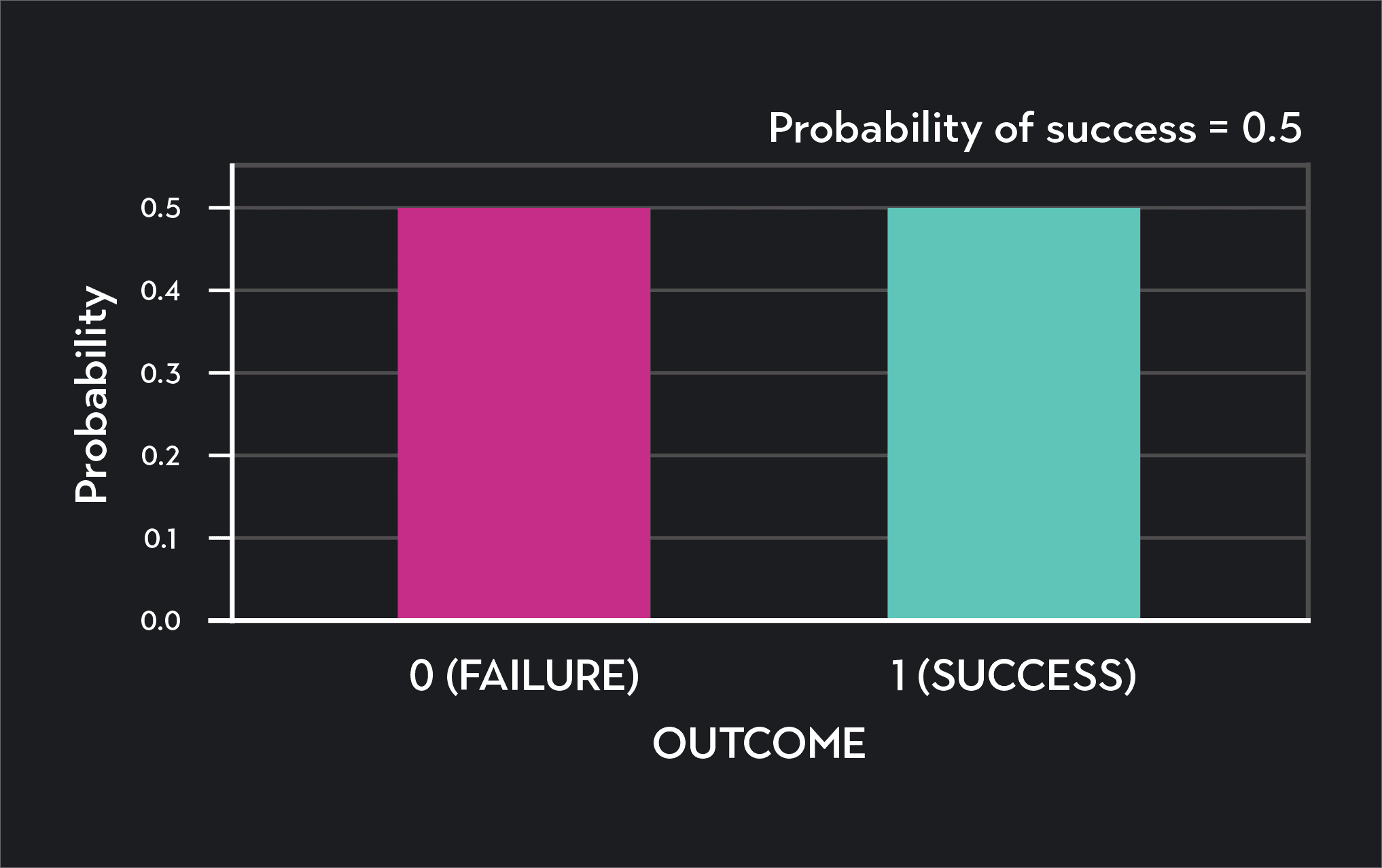
Let’s start with the easiest Bernoulli experiment—that of a coin flip where the probability of success (the coin landing heads) is 0.5, and the probability of failure (the coin landing tails) is 0.5. We’ll see that the distribution depends not just on these probabilities, but also on the number of trials $n$.

The probability distribution for flipping a fair coin once (n=1) looks like this. This is the probability distribution for a single Bernoulli trial. Notice that there is an equal chance of success (heads) and failure (tails). Both outcomes occur with a 50% chance.

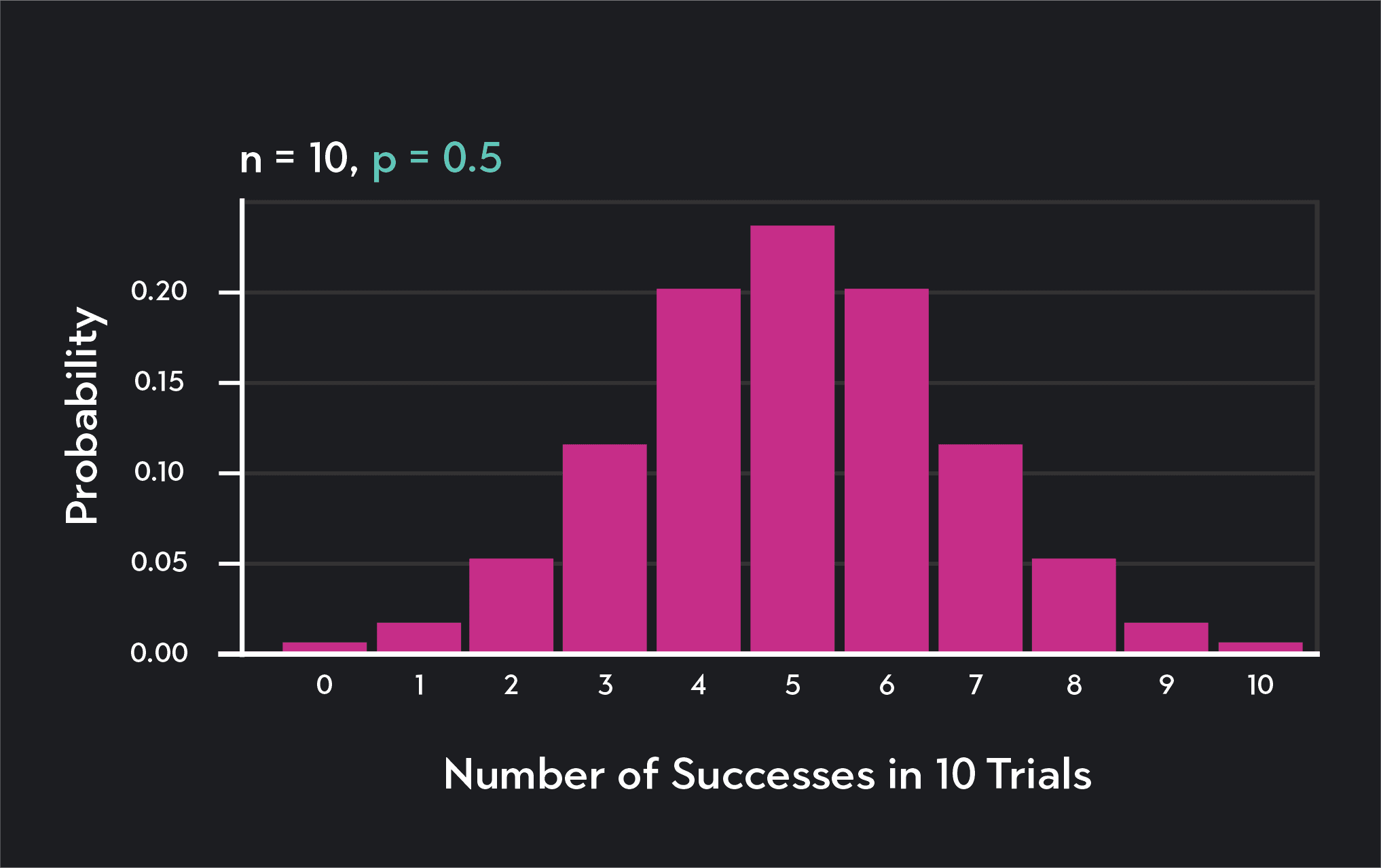
Now, here is what the binomial distribution looks like if we flip the coin ten times (n=10). Notice that the horizontal axis of the graph changes and that there are now ten different possible values for $X$. You could have anything from 0 successes to ten successes across the ten trials.

This particular distribution tells you that after ten coin flips, the probability of getting zero heads (or zero successes) is less than 0.001 (or 0.1%). The probability of 1 success is approximately 0.01 (or 1%), and so on. The mean of this distribution is equal to $np$, which is 10 x 0.5 = 5. This is the expected number of successes after ten flips.

Example 2: Free Throws

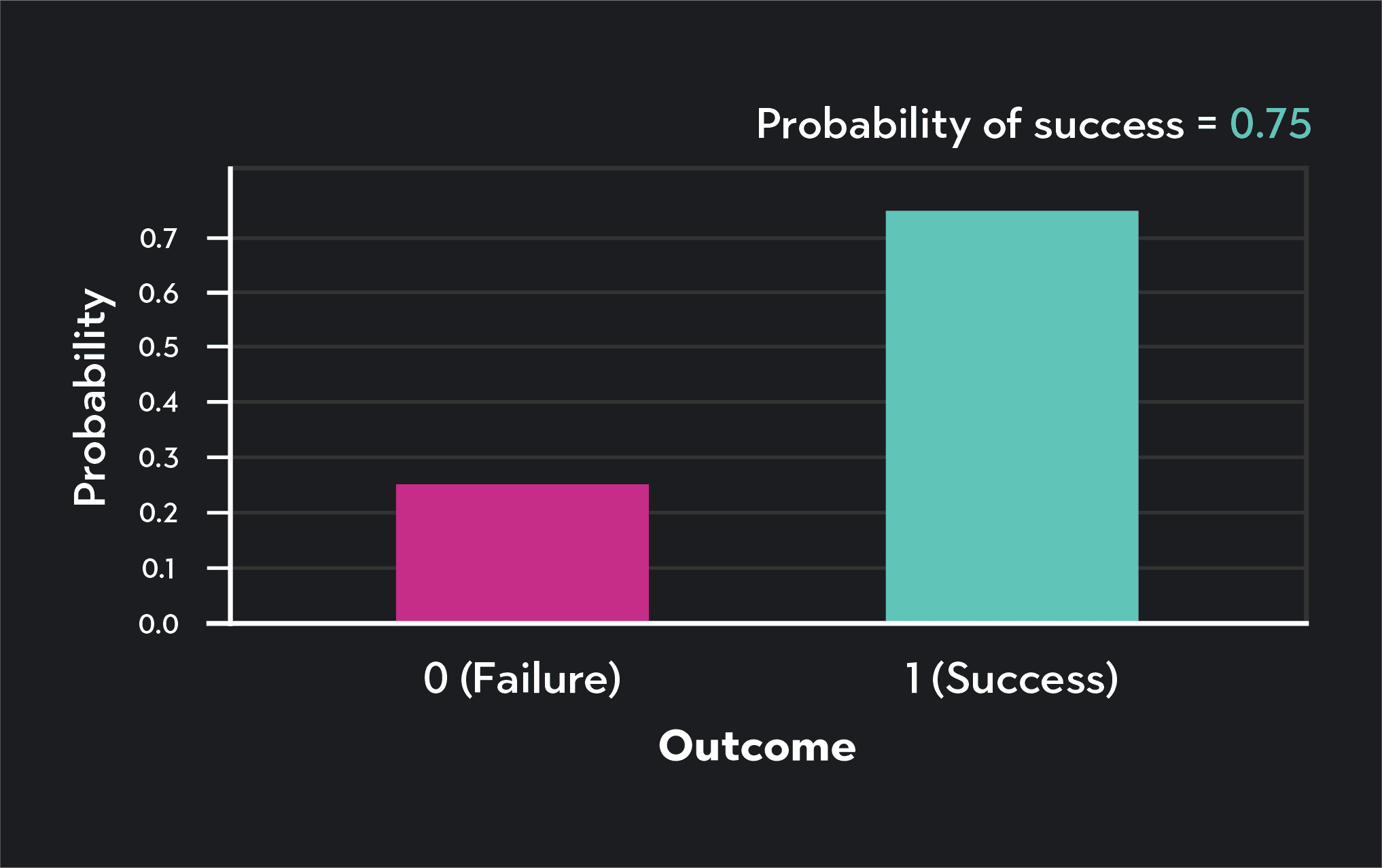
Similarly, here is the Bernoulli distribution of shooting a single free throw when your free throw percentage is 75% (p=0.75). This graph shows that on a single trial, you’ll make the shot with a probability of 0.75, and you will miss (i.e., fail) with a probability of 1-0.75 or 0.25.

Below is the binomial distribution showing the probability of making $x$ number of free throws after 20 shots. We still assume the free throw percentage to be p = 0.75.

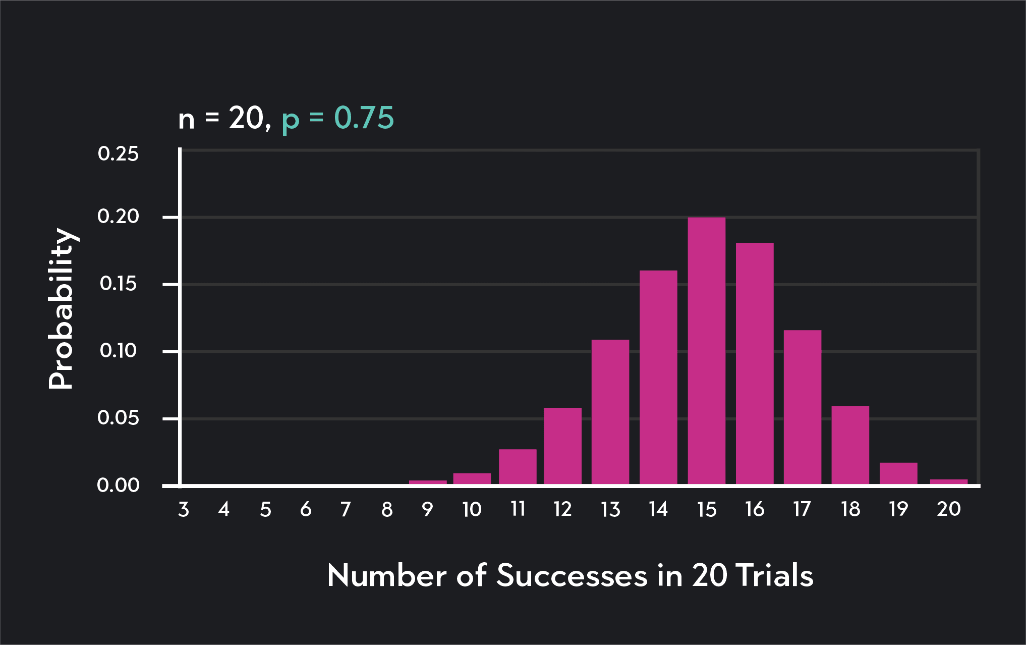
Notice that this distribution looks quite different from the binomial distribution for ten repeated coin flips. That’s because both parameters ($n$ and $p$) have changed. The probability of success is now higher, so the distribution is left-skewed. If instead, $p$ was smaller than 0.5, the distribution would be right-skewed. The number of trials, $n$, has increased, so the total number of successes along the horizontal axis has also increased.

This distribution shows that when your free throw percentage is 0.75, the probability of making less than half of your shots is fairly low. The chance of making exactly 16 out of 20 shots is about 19%. The mean of the distribution is np = 0.75x20 =15, which means you can expect to make 15 out of 20 shots on average.

Binomial Distribution Examples

You can use the binomial distribution to calculate numerous statistics and probabilities. Here are some more examples.

Example 1: Coin Flips

Question 1

Assume you are playing a game where a fair coin is tossed 50 times. What is the probability of getting only 20 tails?

Answer 1

Here you can use the probability mass function to calculate the probability. All you need to do is plug in the relevant values for $n$, $p$, and $x$. Where n=50 trials, p = 0.50, and x = 20 successes.

Question 2

What is the standard deviation for a binomial distribution representing a fair coin that’s tossed 25 times?

Answer 1

To answer this question, you need to plug the values of $n$ and $p$ into the equation for the standard deviation of a binomial distribution.

Example 2: Free Throws

Question 3

A WNBA player has an 85% free throw percentage. If the player is expecting to shoot 250 free throws in a season, how many should she expect to make?

Answer 3

This question asks for the expected value or mean of the binomial distribution. We know the mean is equal $np$, so we simply plug the relevant values of $n$ and $p$ into the equation to get the answer.

Example 3: Spinning a Roulette Wheel

This next example requires converting an experiment with more than two outcomes into a Bernoulli experiment.

A roulette wheel has 38 pockets with different numbers and two different colors (red and black). Although there are 38 unique outcomes when you spin a roulette wheel, as someone betting on where the ball will land, the outcomes you care about are simply “success” or “failure,” win or lose.

Question 4

Suppose you want to bet that a roulette ball will land on a low number (1-18). Using a binomial distribution, what is the probability of winning exactly 12 out of 20 times?

Answer 4

The roulette wheel has 38 pockets, and you are betting on the chances of the ball landing in one of 18 pockets. Your probability of success on each trial is $p$=18/38 = 0.4737. Your probability of failure is (1-p) = 0.5263. You are spinning the wheel 20 times, so $n$ = 20. Now that you have the parameters you need, simply plug them into the probability mass function to find the answer.

Calculating Binomial Probabilities Using R

To calculate a binomial probability using R, you can use the following commands.

To find an exact probability, $P(𝘟=x)$, use the dbinom command.

For example, what is the probability of making 20 out of 30 free throws with a 60% free throw percentage? $P(𝘟=20)$

> dbinom(20, size=30, prob=0.6)

[1] 0.115

To find the probability that $X$ is less than or equal to some value, $P(X≤x)$, use the pbinom command. This command gives you cumulative probabilities.

For example, what is the probability of making 20 or fewer shots out of 30 free throws, assuming your free throw percentage is 60%? P(X≤20)

> pbinom(20, size=30, prob=0.60)

[1] 0.824

To find the probability that $X$ is greater than some value, $P(X>x)$, use the pbinom command. Since this function gives cumulative probabilities to the left of some value, you need to subtract the probability that $X≤x$ from 1 in order to find the probability you are looking for.

For example, what is the probability of making at least 20 out of 30 free throws when your free throw percentage is 60%? $P(X>20)$

>1- pbinom(20, size=30, prob=0.60)

[1] 0.176

You now have the edge over most people in betting on coin flips and calculating free throw percentages. Statistics is filled with useful probability distributions.

Explore Outlier's Award-Winning For-Credit Courses

Outlier (from the co-founder of MasterClass) has brought together some of the world's best instructors, game designers, and filmmakers to create the future of online college.

Check out these related courses:

Intro to Statistics

How data describes our world.

Explore course

Intro to Statistics

How data describes our world.

Explore course

Intro to Microeconomics

Why small choices have big impact.

Explore course

Intro to Microeconomics

Why small choices have big impact.

Explore course

Intro to Macroeconomics

How money moves our world.

Explore course

Intro to Macroeconomics

How money moves our world.

Explore course

Intro to Psychology

The science of the mind.

Explore course

Intro to Psychology

The science of the mind.

Explore course