A residual (or error) is the difference between the predicted value of your data and the actual value of your data. Often we denote a residual with the lower case letter e.
Calculating residuals is easy. You can find residuals using the following equation.
e=y−y^
e is the residual for a given observation of a variable
y is the actual or observed value of y
y^ is the predicted value of y
Example and Practice Finding Residuals
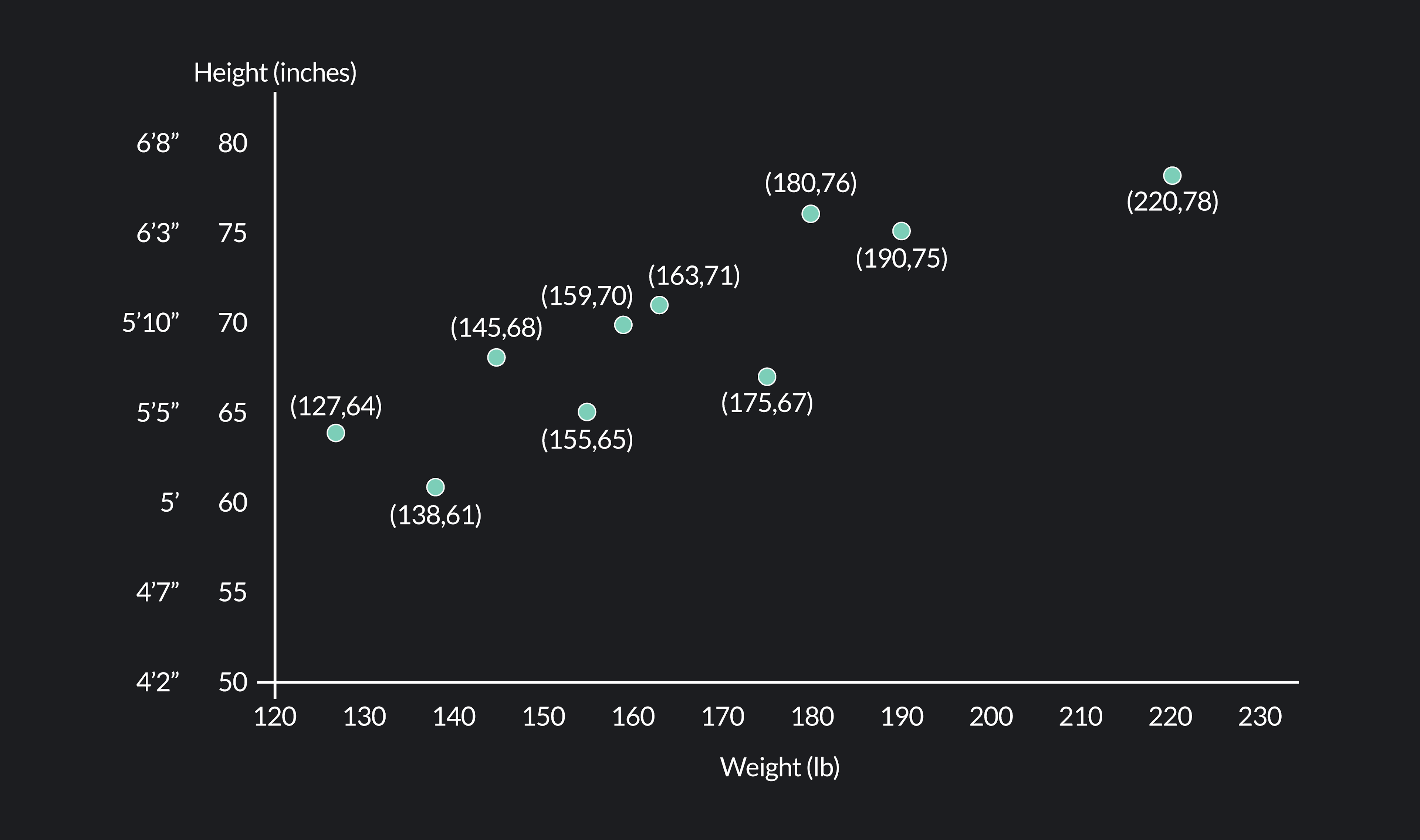
The following table contains a data set with the weight and height of ten individuals. Then, we’ve plotted the data on a scatter plot with weight on the horizontal axis (the x-axis) and height on the vertical axis (the y-axis).
Weight (x)
Height (y)
127 lbs
64 in
138 lbs
61 in
145 lbs
68 in
155 lbs
65 in
159 lbs
70 in
163 lbs
71 in
175 lbs
67 in
180 lbs
76 in
190 lbs
75 in
220 lbs
78 in
In statistics, you will often use a model to approximate the relationship between two variables. This model could take the form of a line (a linear model) or a curve (a non-linear model).
Linear Model
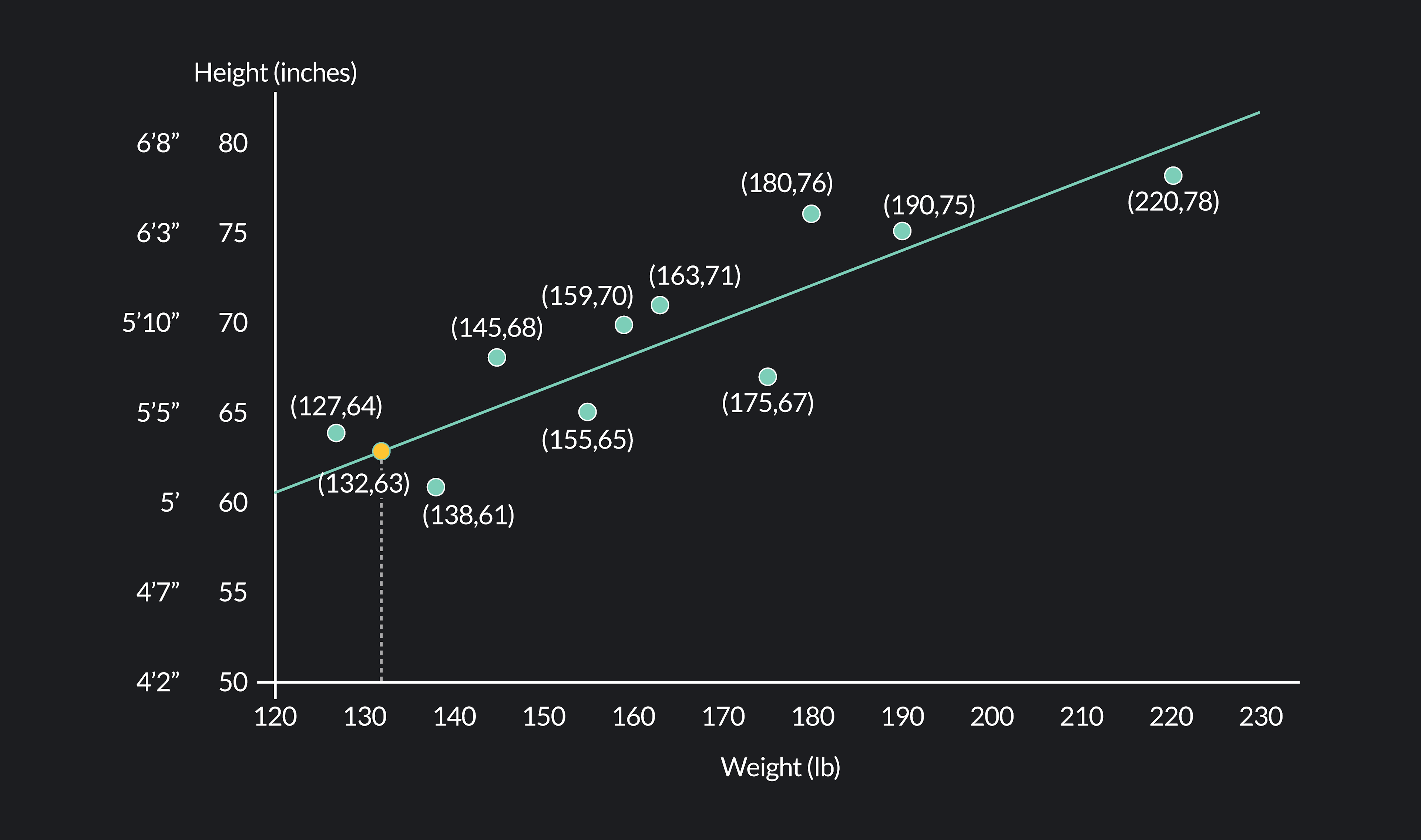
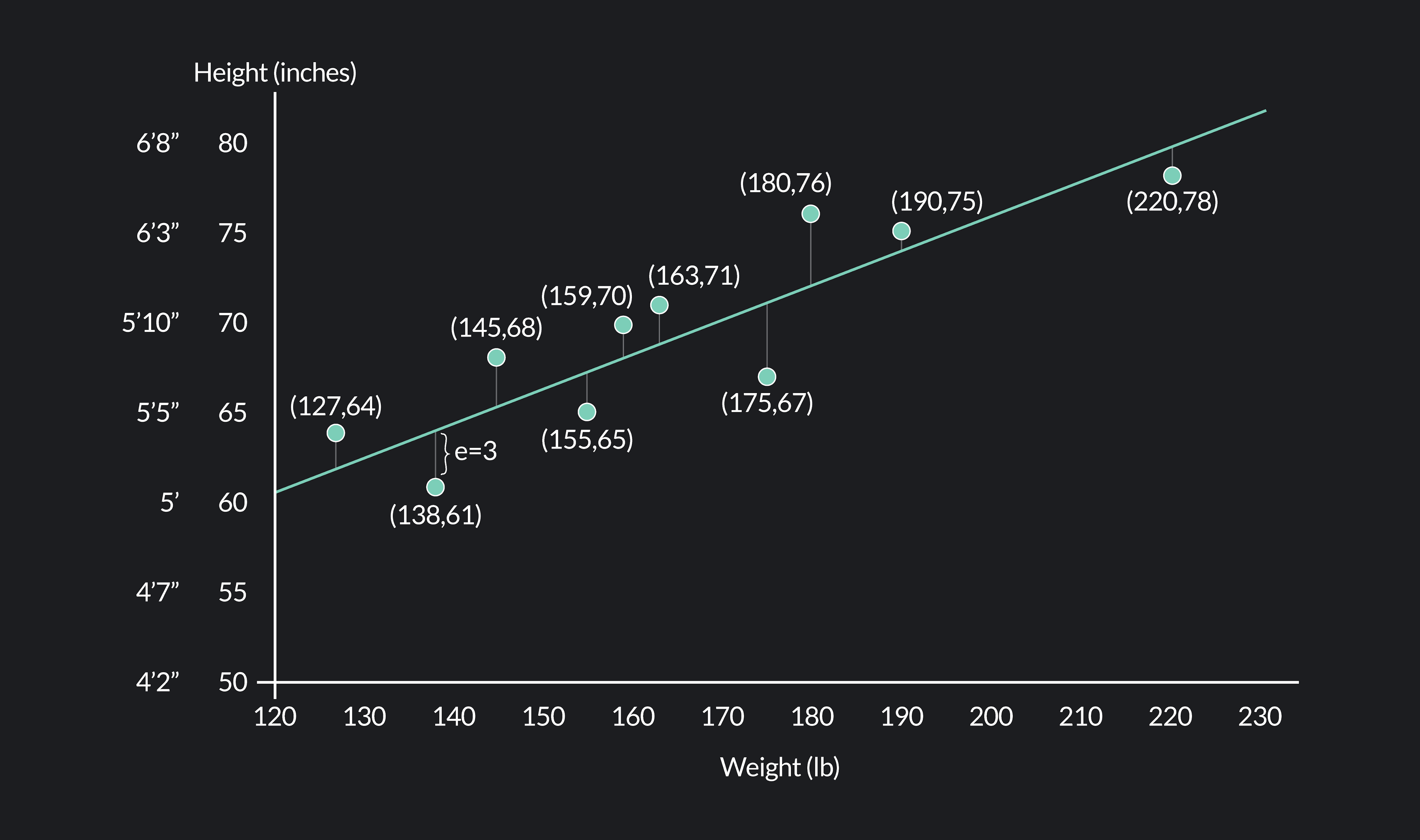
In this example, we’ll use a linear model to approximate the relationship between the weights and heights in our data set (the linear model is represented by the green line in the figure below).
Using this model, we can now estimate a person’s height given their weight. For example, if we know a person weighs 132 lbs, our model estimates 63 inches or 5 ft 3 inches for the person’s height.
Notice that the model does not perfectly line up with the data. If it did, every point on the scatter plot would fall directly on the line, and the predictions of the model would match the data perfectly. Instead, we see a discrepancy between the data and the heights predicted by the model.
For example, take a look at the actual and predicted heights associated with a weight of 138 lbs. Our model predicts that a person weighing 138 lbs will be 64 inches tall, but the data shows a person weighing 138 lbs who is only 61 inches tall.
For any given weight, the difference between the actual height we observe in the data (y) and the predicted height given by the model (y^) is what we call the residual. For the observed data point (138, 61), the residual is y−y^ = 61-64 = -3.
Note that when the actual value from your data lies below the linear model y < ŷ, you will get a negative residual. When the actual value from your data lies above the linear model y > ŷ, you will get a positive residual. This is because you always subtract the predicted value from the actual value to find the residual.
Here's an explanation of linear regression models from one of our instructors.
Now that you know how to find residuals see if you can find the residuals for the remaining data points. Use the actual and predicted values of y in the second and third columns of the table below to fill out the last column labeled “Residuals (e).”
Weight (x)
Actual Height (y)
Predicted Height (ŷ)
Residuals (e)
127 lbs
64 in
62 in
138 lbs
61 in
64 in
-3
145 lbs
68 in
65.5 in
155 lbs
65 in
67.2 in
159 lbs
70 in
68.1 in
163 lbs
71 in
68.85 in
175 lbs
67 in
72.12 in
180 lbs
76 in
71.2 in
190 lbs
75 in
74 in
220 lbs
78 in
80 in
Answer key: (From top to bottom) 2, -3, 2.5, -2.2, 1.9, 2.15, -5.12, 4.8, 1, -2
Interpreting Residuals
One of the biggest challenges of building a statistical model is deciding which model to use. How do you know whether to use a linear or a non-linear model? If you decide to use a linear model, how do you know what the slope and intercept of the line should be? What is the line of best fit?
Residuals are incredibly useful for determining which models are best suited for a particular data set. Using something called a residual plot graph, we can determine whether a linear or a non-linear model is preferable. We can also use the sum of the squared residuals to find a model that minimizes residuals. We’ll cover both of these topics next!
What is a Residual Plot?
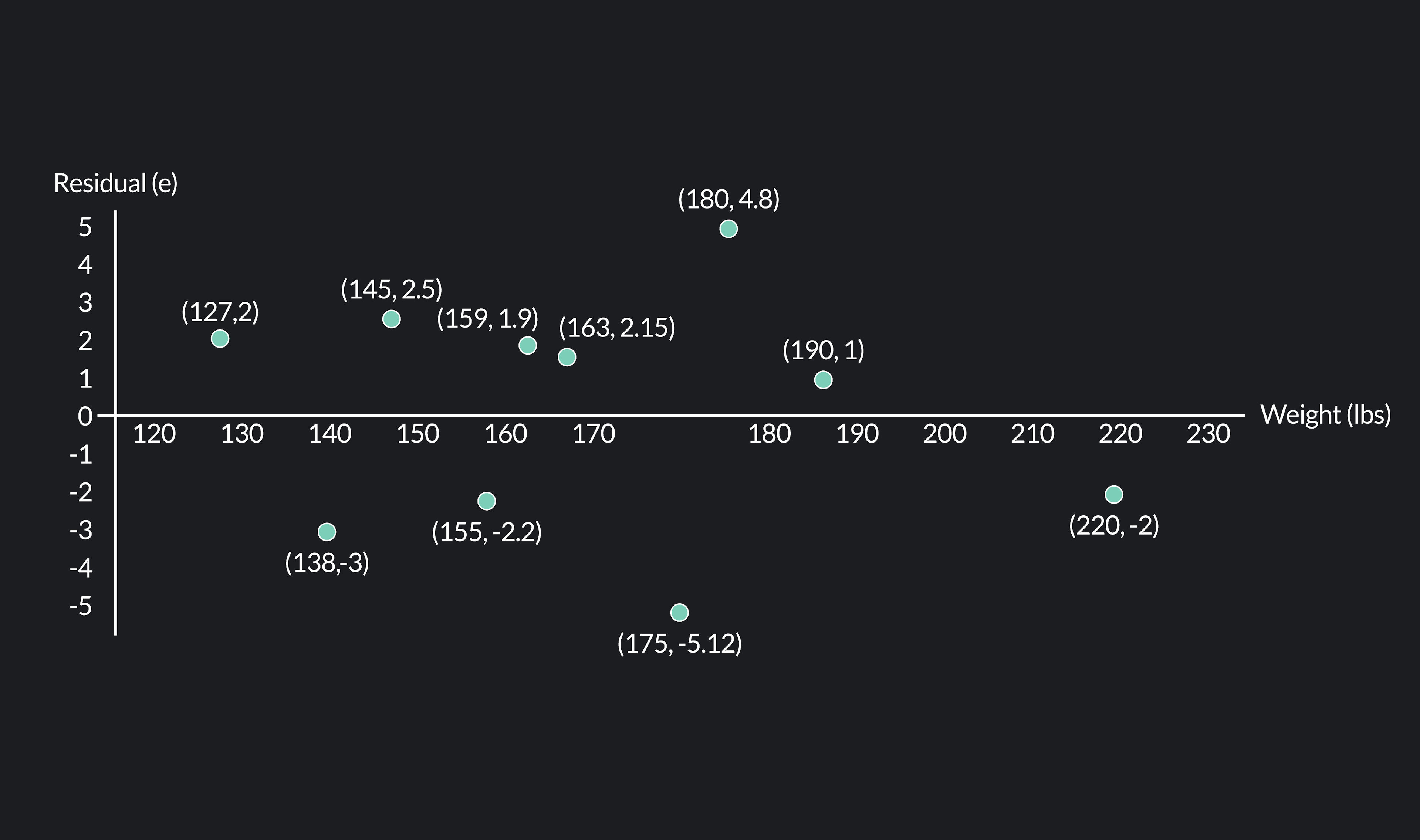
A residual plot is a scatter plot with the residuals of a variable plotted on
the y-axis and the values of the x-variable plotted on the x-axis.
Continuing from our example above, let’s create a residual plot for our data on heights and weights. Earlier, we found that the residuals for our data were: 2, -3, 2.5, -2.2, 1.9, 2.15, -5.12, 4.8, 1, -2. Our residual plot has these residual values plotted against the y-axis, and the observed weights plotted against the x-axis.
You should always use a linear model when there is a linear relationship (either a positive or negative correlation) between your variables. You should use a non-linear relationship when the correlations between the variables change between being positive and negative. Sometimes, a scatter plot of your data will clearly show a linear or non-linear trend, but sometimes the pattern can be more ambiguous. If this is the case, you can use a residual plot to determine which model to use.
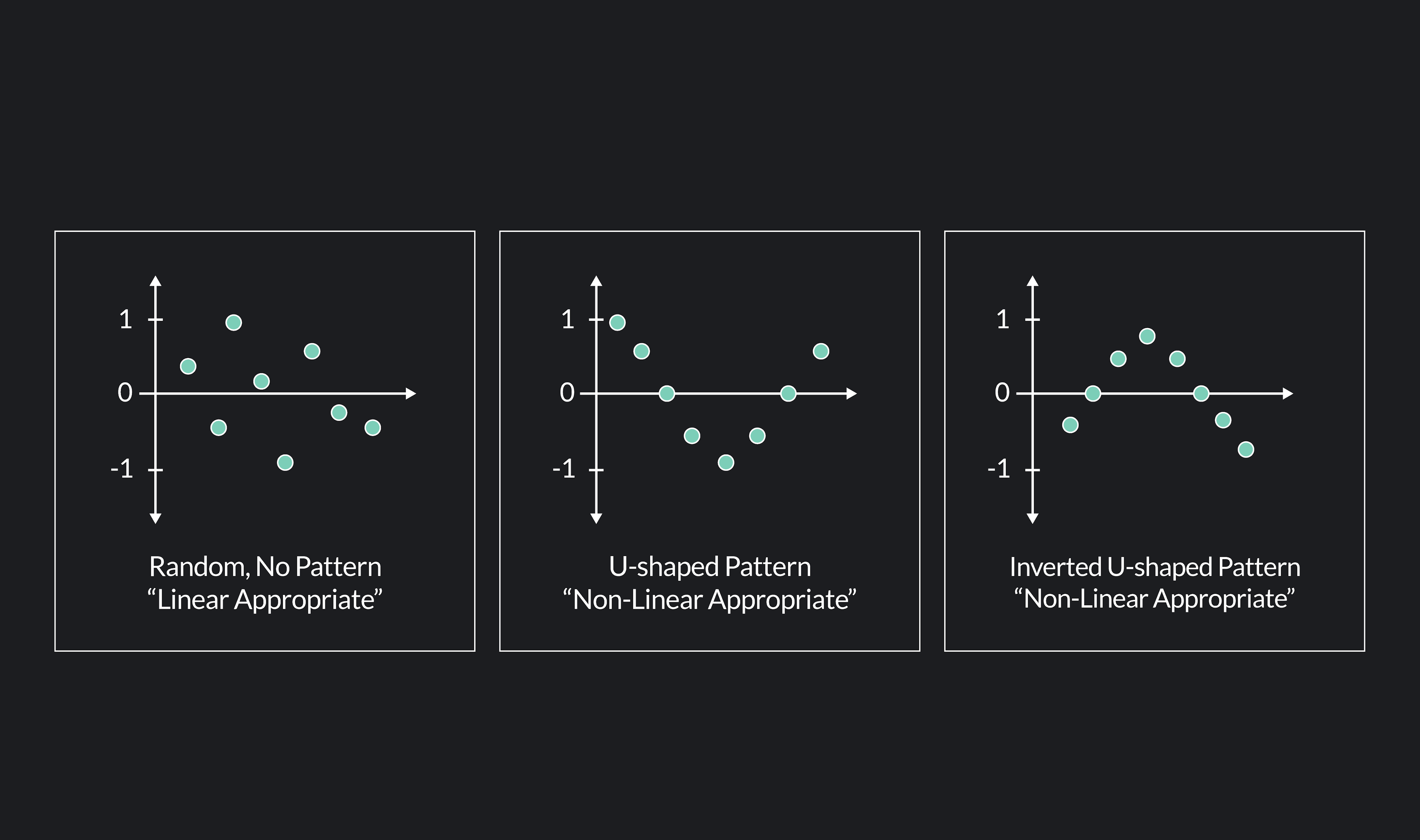
When a residual plot shows the residual values plotted randomly above and below the x-axis, then a linear model is a good fit for the data. This was the case in the residual plot for heights and weights, so we were right to use a linear model instead of a non-linear model.
When the plotted residuals follow a u-shaped pattern or an inverted u-shaped pattern, then a non-linear model is better suited for your data.
Concept of Linear Association and Linear Regression
So far, we have talked a lot about statistical models. These models are called regressions. A linear regression model or regression line is the same thing as the linear models we have been discussing so far. It is a model of the association between two variables — an independent variabley - also called an outcome or response variable) - and a dependent variable x - or explainer variable.
Because a linear regression is a line, we can express linear regressions using the equation for a line.
As you may recall from a geometry class, the equation for a line is y=mx+b, where:
y represents the value of the variable plotted on the y-axis
x represents the value of the variable plotted on the x-axis
m represents the slope of the line
b represents the y-intercept of the line
We use the same equation but with slightly different notation when dealing with linear regression. You’ll often see a linear regression expressed in one of the following ways.
Linear Regression Equation
y^=a+bx
or
y^i=ꞵ0+ꞵ1xi
y^ or y^i is the predicted value of y
a or ꞵ0 is the vertical intercept of the linear regression
b or ꞵ1 is the slope of the linear regression (also referred to as the regression coefficient)
x or xi is the value of the x-variable associated with a particular value of y
Residuals and Linear Regressions
Once we’ve determined that a linear regression - as opposed to a non-linear - should be used, we can continue to use residuals to determine which line is the “best fit” for the data.
Ordinary Least Squares
A method that is commonly used for this is called Ordinary Least Squares (OLS) method. In OLS, you choose the linear regression that minimizes the sum of the squared residuals. By doing this, you are essentially minimizing the discrepancies between the data and your model.
We square the residuals because some residuals are positive while others are negative. If we don’t square the residuals, the negative residuals will cancel out the positive residuals in our calculations. The reason why we don’t take the absolute value of the residuals instead of taking the squares is that we want to give more weight to very large residuals and make sure any large residuals are minimized. (A large residual squared will become an even larger number compared to a small residual that is squared.)
Ordinary Least Squares (OLS) Regression is
a method for finding a linear regression where the regression used is the one that minimizes the sum of the squared residuals.
OLS Regression Method:minΣ(en)2
Let’s have another look at the scatter plot and linear regression we used for our weights and heights example.
Remember, the basic idea behind OLS is that we want to minimize the sum of the squared residuals. On our graph, the vertical distance of the lines represents the residuals.
If we were to use the OLS method, we would square the distance of each of the red lines and add all of the squared distances together. According to the OLS method, the regression we should choose is the one with the smallest squared distance!
Summary and Applications of Residuals
To recap, a residual tells us how well a model fits the data. It is the difference between the actual value of a variable y and the predicted value of a variable y^.
In regression analysis, residuals can be used to determine whether a linear or a non-linear regression should be used to model the data. This determination can be made using a scatter plot of residuals called a residual plot. Residuals can also be used to determine which regression is the best fit for your data.
A common method for finding a model of “best fit” is the OLS method. In OLS, you choose the regression that minimizes the sum of the squared residuals.
Outlier (from the co-founder of MasterClass) has brought together some of the world's best instructors, game designers, and filmmakers to create the future of online college.