Calculating p-Value in Hypothesis Testing

In This Article

1. What Is a p-Value?

2. Calculating p-Values for Discrete Random Variables

3. Calculating p-Values for Continuous Random Variables

What Is a p-Value?

A p-value (short for probability value) is a probability used in hypothesis testing. It represents the probability of observing sample data that is at least as extreme as the observed sample data, assuming that the null hypothesis is true. 

In a hypothesis test, you have two competing hypotheses: a null (or starting) hypothesis, $H_0$ and an alternative hypothesis, $H_a$. The goal of a hypothesis test is to use statistical evidence from a sample or multiple samples to determine which of the hypotheses is more likely to be true. The p-value can be used in the final stage of the test to make this determination.

Interpreting a p-value

Because it is a probability, the p-value can be expressed as a decimal or a percentage ranging from 0 to 1 or 0% to 100%. The closer the p-value is to zero, the stronger the evidence is in support of the alternative hypothesis, $H_a$.

Reject or Fail to Reject the Null Hypothesis?

When the p-value is below a certain threshold, the null hypothesis is rejected in favor of the alternative hypothesis. This threshold is known as the significance level (or alpha level) of the test. 

The most commonly used significance level is 0.05 or 5%, but the choice of the significance level is up to the researcher. You could just as easily use a significance level of 0.1 or 0.01, for example. Remember, however, that the lower the p-value, the stronger the evidence is in support of the alternative hypothesis. For this reason, choosing a lower significance level means that you can have more confidence in your decision to reject a null hypothesis.

When the p-value is greater than the significance level, the evidence favors the null hypothesis, and the researcher or statistician must fail to reject the null hypothesis.

Calculating p-Values for Discrete Random Variables

As mentioned earlier, the p-value is the probability of observing sample data that’s at least as extreme as the observed sample data, assuming that the null hypothesis is true. 

If your data consists of a discrete random variable, you can map out the entire set of possible outcomes and their respective probabilities in order to calculate the p-value. 

The p-value will then be the sum of three things:

• the probability of the observed outcome

• the probability of all outcomes that are just as likely as the observed outcome

• and the probability of any outcome that is less likely than the observed outcome

Here is an example. 

A stranger invites you to play a game of dice, and claims her dice are fair. The rules of the game are as follows: You roll a single die. If you roll an even number, you count that as a win (or success) and earn $1. If you roll an odd number, you count that as a loss (or failure) and lose $0.80. You can play the game for as many rounds as you like. 

Let’s say you play four rounds of the game, and you lose all four rounds. This leaves you $3.20 poorer than before you started playing.

Given your losses, you may be interested in conducting a hypothesis test. The null hypothesis will be that the dice used in the game are indeed fair and that there is an equal chance of rolling an even or odd number with each roll. Your alternative hypothesis is that the dice are weighted towards landing on odd numbers.

To calculate the p-value, we map all of the possible outcomes of playing four rounds of the game. In each round, there are only two possible outcomes (odd or even), and after four rounds, there are a total of $2^4$, or 16, outcomes. If we assume the null hypothesis is true—that the dice are fair)—each of these outcomes is equally likely, with a probability of 1/16.

Since we are only concerned about the total number of wins and losses, and not concerned at all with their order, the outcomes and probabilities we care about are the following:

• the probability of getting 4 wins and 0 losses = 1/16

• the probability of getting 3 wins and 1 loss = 4/16

• the probability of getting 2 wins and 2 losses = 6/16

• the probability of getting 1 win and 3 losses = 4/16

• the probability of getting 0 wins and 4 losses = 1/16

To calculate the p-value, we sum up the following:

• the probability of the observed outcome (0 wins and 4 losses) 

• the probability of any outcome that is just as likely as the observed outcome (4 wins and 0 losses)

• the probability of any outcome that is less likely than the observed outcome (in this example, there are no outcomes that are less likely than the observed outcome, so this value is zero)

p-Value =  1/16 + 1/16 = 1/8 or 0.125

The p-value we found is 0.125. Surprisingly, this is still well above a 0.05 significance level. It is even above a 0.10 (or 10%) significance level. Regardless of which of these thresholds you choose, you must fail to reject the null hypothesis. In other words, despite four losses in a row, the evidence still favors the hypothesis that the dice are fair! It may be a different story if you experience 10 or even 5 losses in a row. Calculate the p-value to find out!

Calculating p-Values for Continuous Random Variables

When the hypothesis test involves a continuous random variable, we use a test statistic and the area under the probability density function to determine the p-value. The intuition behind the p-value is the same as in the discrete case. Assuming that the null hypothesis is true, we are calculating the probability of observing sample data that is at least as extreme as the sample data we have observed.

Let’s take a look at another example.

Say you have an orange grove, and you’re convinced that your oranges now grow larger than when you first started growing citrus. You happen to know that the standard deviation of the weights of your oranges, $\sigma$, is equal to 0.8 oz. This is the perfect opportunity to conduct a hypothesis test.

Your null hypothesis, in this case, is that the mean weight of your oranges has remained unchanged over the years and is equal to 5 oz (the null hypothesis typically represents the hypothesis that you are trying to move away from). Your alternative hypothesis is that the average weight of your oranges is now greater than 5 oz.

Because you can’t weigh every orange in your grove, you pick a large random sample of oranges (with a sample size of 100), weigh those, and observe that the average weight in your sample, $\overline x$, is equal to 5.2 oz. 

Does this result support the null hypothesis or the alternative hypothesis? It’s not immediately clear. By pure chance, you could have had a handful of extra-large oranges in your sample, and this could have pushed your sample mean above a population mean of 5 oz. Alternatively, the sample mean could indicate that the population mean is, in fact, greater than 5 oz. 

Here is where we begin the hypothesis test. We’ll conduct the test at a 0.05 significance level.

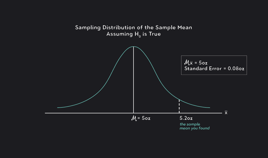
We start by asking the following question: Assuming that the null hypothesis is true, how likely or unlikely is it to observe a sample mean $\overline x$ = 5.2 oz?

From the central limit theorem, we know that if our sample is randomly drawn and large enough, we can assume that the sampling distribution of the sample means is normally distributed with a mean equal to the true population mean, $\mu$, and a standard error equal to $\frac\sigma{\sqrt n}$. This means that if the null hypothesis is true, the sampling distribution for the sample mean of our orange weights will be normally distributed, with a mean equal to 5 and a standard error equal to 0.08.

From here, we can convert our sample mean of 5.2 into what is known as a test statistic. To do this we use the exact same process we use when calculating standardized units such as z-scores or t-scores. Since we know the sampling distribution is approximately normal, and since we know the population standard deviation ​​$\sigma$ and the standard error $\frac\sigma{\sqrt n}$ of the sampling distribution, we can calculate a Z-test statistic in the same way that we would calculate a z-score (if we did not know $\sigma$, we would use the sample standard deviation, s, to calculate a t-test statistic in the same way that we calculate t-scores).

The test statistic is telling us that if our null hypothesis is true, then our observed sample mean, $\overline x$, is 2.5 standard deviations above the mean of the sampling distribution. To put the p-value to work we can do one of two things.

1. We can calculate the p-value associated with the test statistic. This can be done by finding the area under the standard normal distribution that lies to the right of 2.5. This gives us a p-value of 0.0062. The p-value is telling us that if the null hypothesis is true, we would only observe a sample mean of 5.2 or greater 0.0062 (or 0.62%) of the time. Because this probability is so low, it’s likely that the null hypothesis is false.

Since the p-value of 0.0062 is less than the significance level of 0.05, we can reject the null hypothesis at the 0.05 significance level. We can even reject it at the 0.01 significance level! You’re likely to be right about your oranges: the average weights have likely increased over time.

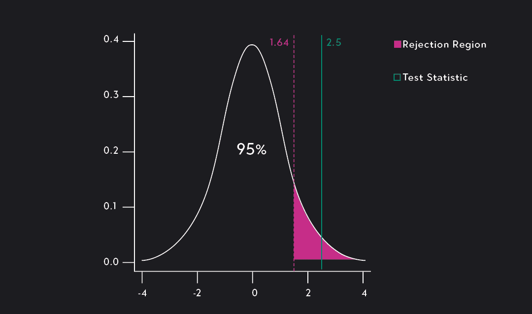
2. If you are familiar with standard normal distributions you may have realized that the significance level of our test (alpha = 0.05) is associated with the 95th percentile of the standard normal distribution. You may also know that the 95th percentile of a standard normal distribution is associated with a Z-score of 1.64.  Since the test statistic 2.5 lies to the right of the Z-score, we can assume that the p-value will be less than 0.05. This is another way to complete the hypothesis test without having to do additional calculations. 

Two-sided, upper-tailed, and lower-tailed hypothesis tests

In the orange grove example above, we conducted an upper-tailed hypothesis test, because the alternative hypothesis $H_a$ was of the form $\mu>\mu_0$. It’s important to know, however, how the calculation of p-values differs when you have a two-tailed or a lower-tailed hypothesis test.

For a two-tailed test (when the alternative hypothesis, $H_a$, stipulates that a population parameter is ≠ to some number), the p-value is equal to twice the probability associated with the test statistic. If we had conducted a two-tailed test in the orange grove example ($H_a$: $\mu\neq5$), the p-value would be equal to the probability that $\overline x$ was greater than 2.5 plus the probability that $\overline x$ is less than -2.5. Because the standard normal is symmetric about the mean, this is equal to (0.0062 * 2 = 0.0124).

For a lower-tailed test (when the alternative hypothesis, $H_a$, stipulates that a population parameter is ≤ to some number) the process is similar to the upper-tailed test, but the p-value will be the probability of getting a sample statistic that lies to the left of the test-statistic, rather than to the right of it. 

Explore Outlier's Award-Winning For-Credit Courses

Outlier (from the co-founder of MasterClass) has brought together some of the world's best instructors, game designers, and filmmakers to create the future of online college.

Check out these related courses:

Intro to Statistics

How data describes our world.

Explore course

Intro to Statistics

How data describes our world.

Explore course

Intro to Microeconomics

Why small choices have big impact.

Explore course

Intro to Microeconomics

Why small choices have big impact.

Explore course

Intro to Macroeconomics

How money moves our world.

Explore course

Intro to Macroeconomics

How money moves our world.

Explore course

Intro to Psychology

The science of the mind.

Explore course

Intro to Psychology

The science of the mind.

Explore course