
Statistics
A Guide To Understand Negative Correlation
This overview is about negative correlation, its definition, its importance, how to determine it, and differences between positive and zero correlation.
Sarah Thomas
Subject Matter Expert

Statistics
08.01.2023 • 6 min read
Subject Matter Expert
Learn about logarithmic regression and the steps to calculate it. We’ll also break down what a logarithmic function is, why it’s useful, and a few examples.
In This Article
Have you ever wondered how scientists and mathematicians determine the relationship between two variables that don't appear to have a linear relationship? Enter logarithmic regression, a powerful data analysis tool that can help us make sense of complex data.
In this article, we'll explore the basics of logarithmic regression, including how it works, when to use it, and how to interpret the results.
A logarithm is a mathematical function that tells you the power to which a base number, , needs to be raised to produce a given value.
For example, if you want to know the power to which the number 3 needs to be raised to produce the number 81, you would find . In this case, the log function tells you that 3 must be raised to the power of 4 to get 81.
Logarithmic functions are an inverse function of exponential functions.
When working with logarithms, you’ll often run into logarithmic functions that use the irrational number —also known as Euler’s number—or the number 10 as base numbers.
A logarithm that uses e as a base number is called a natural logarithm. Natural logarithms are often written as ln(x) instead of . Similar to the general form of logarithms, if , then =.
A logarithmic function that uses 10 as the base number is called a base 10 logarithm or a common logarithm.
Regression is a statistical method we use to study the relationship between a dependent variable, Y, and one or more independent variables, . The dependent variable might also be called a response variable, and the independent variables are often called predictor variables.
The most basic form of regression is a linear regression, where the relationship between the dependent and independent variables is linear i.e., the relationship can be modeled using a straight line.
When the relationship between variables in your data is non-linear, we need to use a nonlinear regression or a modified version of the linear regression model. A logarithmic regression is a modified linear regression that includes one or more logged variables, where “logged variable” simply means taking the logarithm of a variable.
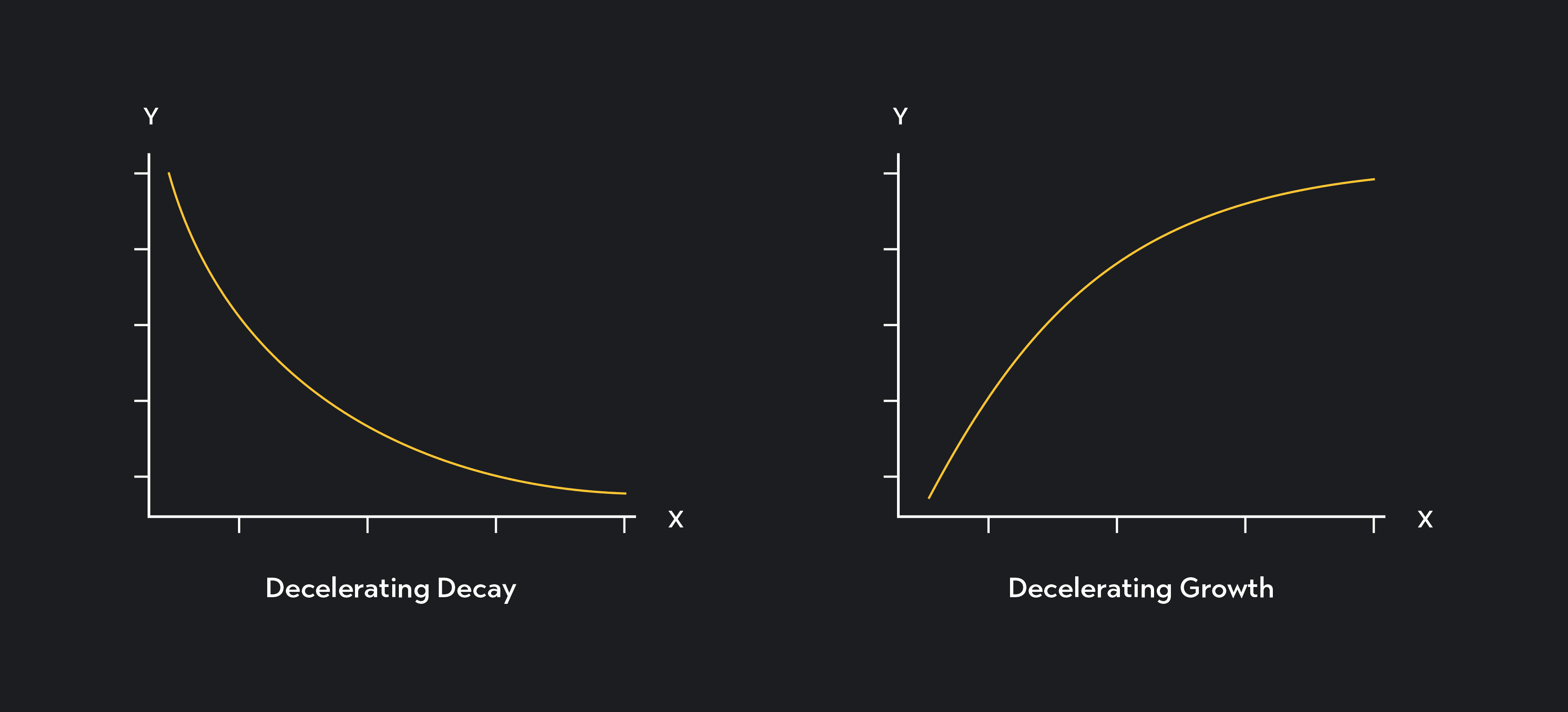
Logarithmic regressions come in handy when your independent and dependent variables follow a nonlinear relationship matching the pattern of decelerating growth or decay. If your dependent variable increases or decreases rapidly at first as the independent variable decreases, but the rate of that increase or decrease gradually slows, you should consider using a logarithmic regression.
Using logged variables in your regression lets you capture the non-linear relationship between your variables while maintaining a regression model that is linear in the parameters—or regression coefficients—of the model.
Another case to use a logged variable is when you are dealing with a variable highly skewed (to the right) and follows a distribution called a log-normal distribution. By performing a log transformation on a highly skewed variable, you can convert the variable into one with an approximately normal distribution. In general, if a variable follows a log-normal distribution, then the log of that variable would follow a normal distribution.
Three types of logarithmic regressions exist. In each type, you take the natural log, ln(x), of one or more of the variables in the regression equation.
In a linear-log model, you perform a log transformation on the independent variable.
In a log-linear model, you perform a log transformation on the dependent variable.
In a log-log model, you perform a log transformation on both the dependent and independent variables.
In a simple linear regression, the regression coefficient gives us the estimated change in Y that results from a one-unit change in the independent variable X. The coefficient, in this case, is measured in units of Y, so if equals 3 and Y is measured in dollars, you would interpret the coefficient as: a one-unit increase in X results in a $3.00 increase in Y.
In a logarithmic regression, the same logic applies, but the interpretation of the coefficient is somewhat different.
In a linear-log model, like the one shown below, the regression coefficient gives you the estimated change in Y associated with a one-unit increase in ln(X).
While it’s difficult to interpret a one-unit increase in a logged term, a benefit of using logged variables in a regression is that the coefficient can be interpreted in terms of percentage changes. In the linear-log case, we can say that 1a p% increase in X results in an estimated change in Y that equals:
As an approximation, we can also say that a one-percent increase in X is associated with a increase in Y.
In a log-linear model, you can interpret the regression coefficient as the estimated percentage change in Y associated with a one-unit increase in X.
In this case, the percentage change is measured on a scale from 0-1. For example, a of 0.12 tells you that Y is estimated to increase by 12% in response to a one-unit increase in X.
In a log-log model, we can interpret the regression coefficient as the percentage change in Y that results from a one percent increase in the independent variable.
Unlike the log-linear case, the percentage change in the log-log model is measured on a scale of 0-100. So if =3.5, for example, Y is estimated to increase by 3.5% in response to a 1% increase in X. You will sometimes hear this type of coefficient being called elasticity, since elasticity measures the percentage change in one variable in response to a percentage change in another.
Below are steps you can follow to calculate a linear-log model.
Suppose you have data on income—measured in thousands of dollars per year—and life expectancy—measured in years. Start by entering or uploading your data into a statistical program like R, Stata, Excel, or Desmos. For this example, we would likely use income to predict life expectancy, so your x-values will be income and your y-values will be life expectancies.
Next, plot your data on a scatterplot and check to see whether it’s appropriate to use linear-log model. Remember, logarithmic regression is used in cases where the relationship between X and Y matches the pattern of decelerating growth or decelerating decay.
Finally, use your software to fit a linear-log function of the form to your data.
Here is a solved example of how to build the same linear-log regression we discussed using Desmos. To do this, we are using a hypothetical dataset on income and life expectancy.
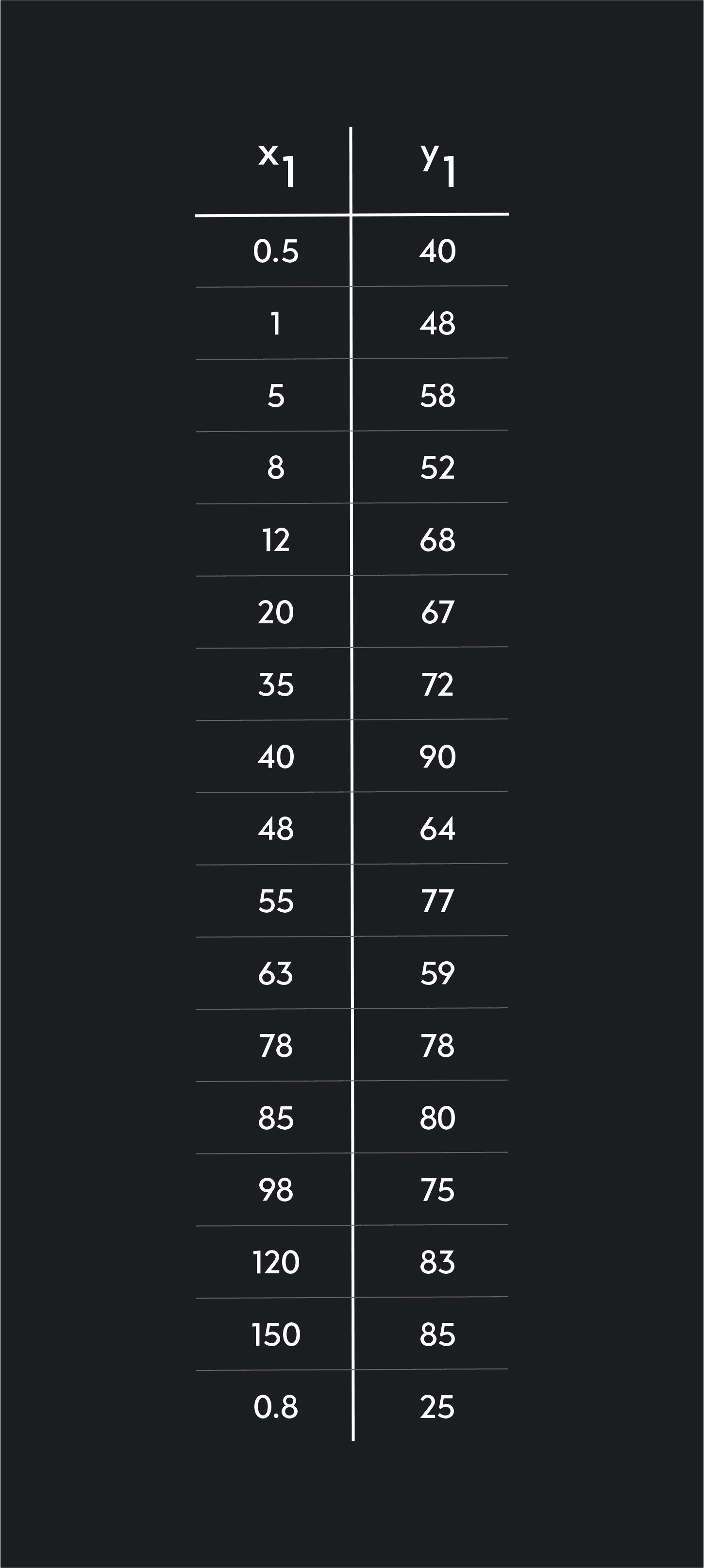
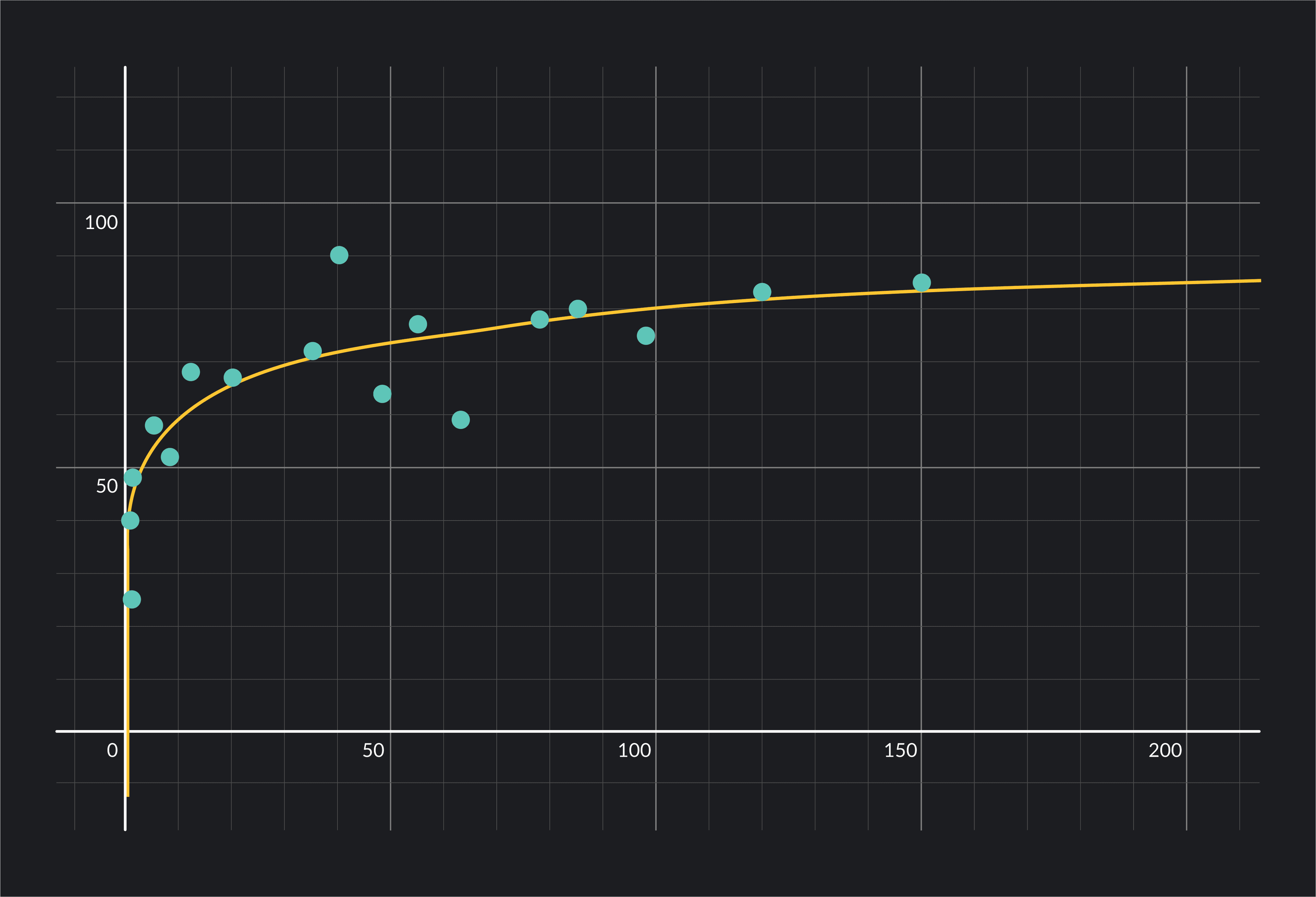
We start by entering or uploading our data into Desmos as a table with representing annual income measured in thousands of dollars and representing life expectancy in years.
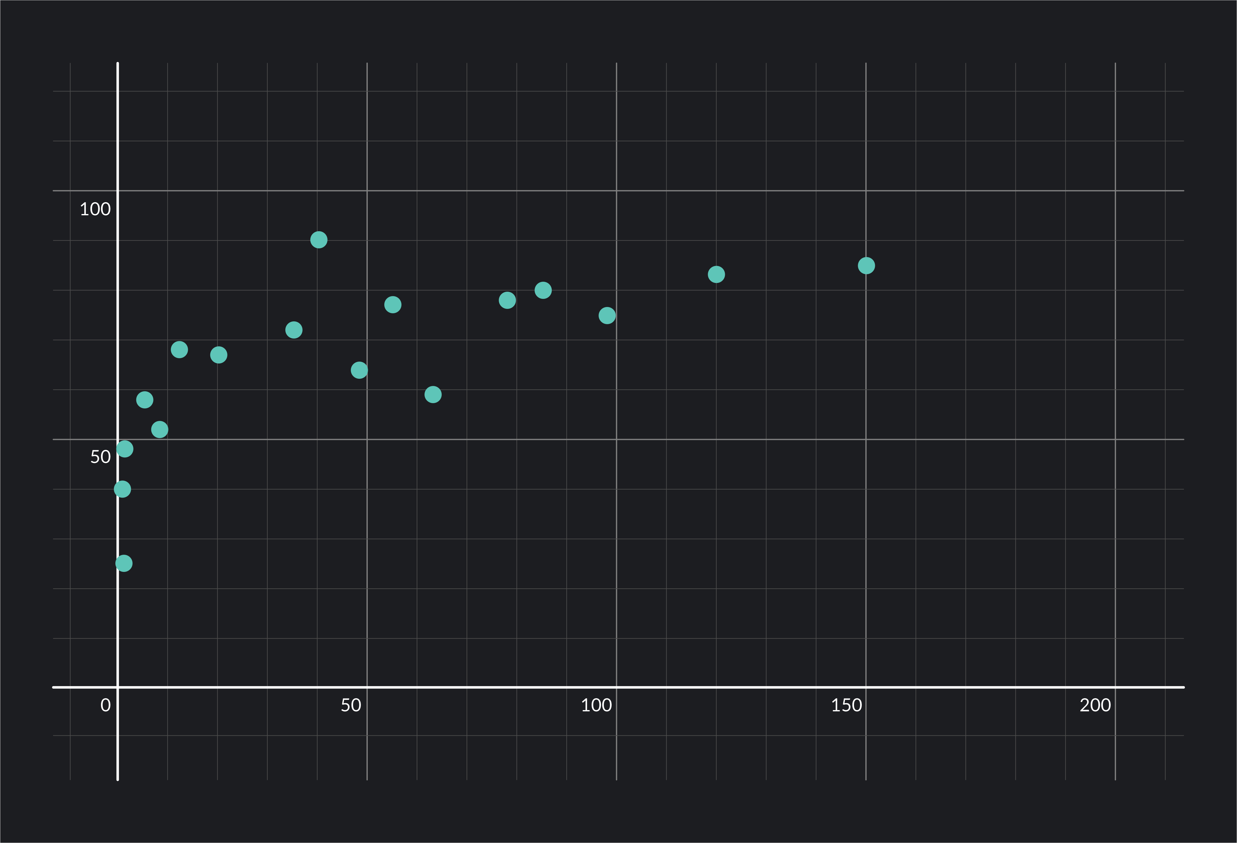
Next, we click on the grey circular icon next to in the data table to plot the data points on a scatter plot. We check to see that data is nonlinear and matches the pattern of decelerating growth or decay. In this case, we see that the data seems to match an increasing logarithmic function. Life expectancy increases with age, but it does at a decelerating rate.
Finally, we fit a linear-log function to the data by entering the following equation into Demos’ command line: . This will fit a curved line to the data and will show you your regression results.
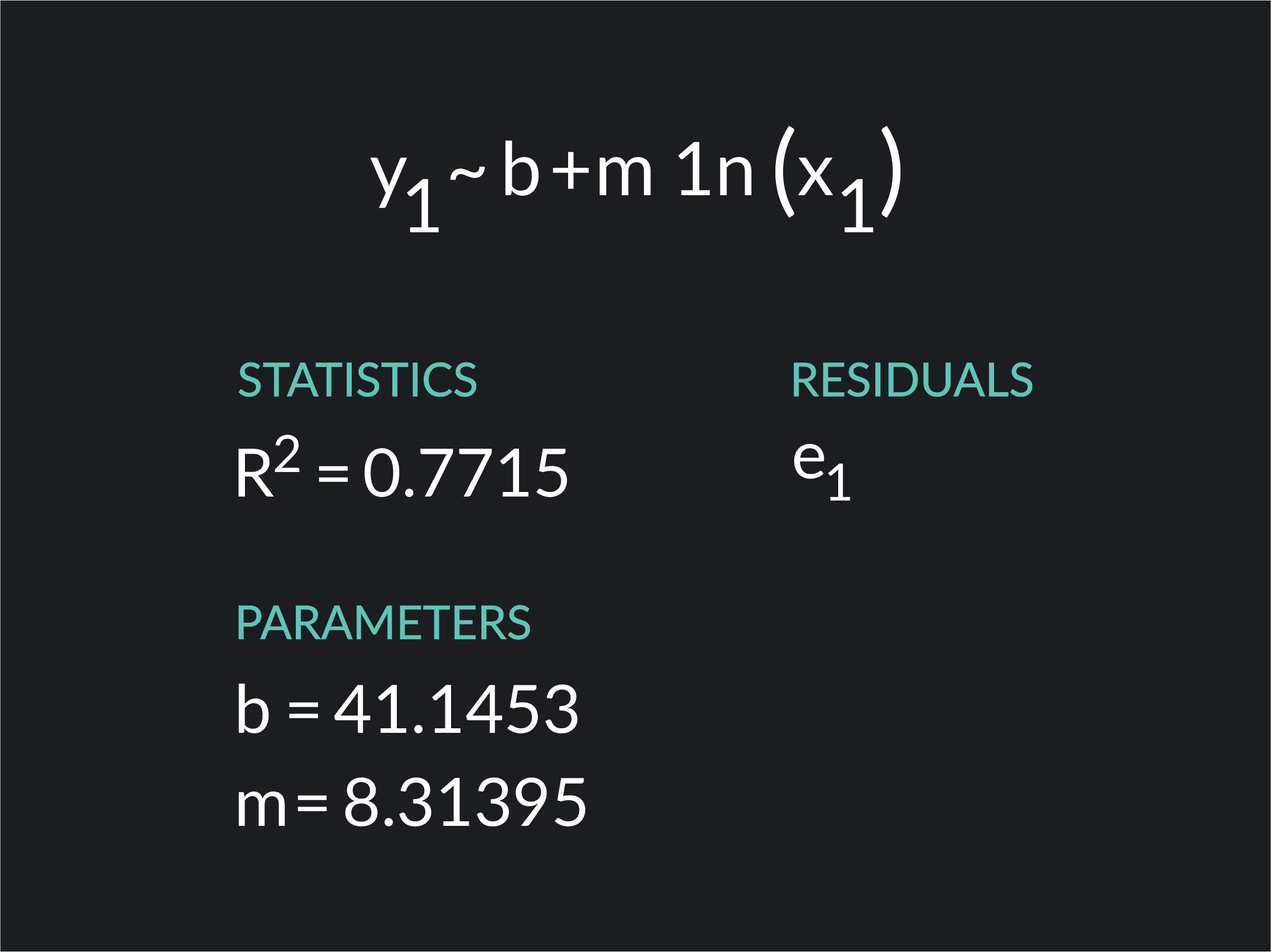
Desmos uses different notation for regressions than what we have used so far. In the Desmos equation, represents the intercept and represents the coefficient on .
The results show that the regression coefficient =8.31395.
Based on what you learned earlier about interpreting coefficients, we can say the following: a one percent increase in income is associated with a or increase in life expectancy . Or, as income increases by 1%, our model estimates life expectancy will increase by 0.0831 years.
Outlier (from the co-founder of MasterClass) has brought together some of the world's best instructors, game designers, and filmmakers to create the future of online college.
Check out these related courses:


Statistics
This overview is about negative correlation, its definition, its importance, how to determine it, and differences between positive and zero correlation.
Subject Matter Expert

Statistics
Learn what the interquartile range is, why it’s used in Statistics and how to calculate it. Also read about how it can be helpful for finding outliers.
Subject Matter Expert

Statistics
This article explains what a test statistic is, how to complete one with formulas, and how to find the value for t-tests.
Subject Matter Expert