Coefficient Regression: Definition, Formula, and Examples

In This Article

1. What Is a Regression Coefficient?

2. Applying the Regression Coefficient

3. Regression Coefficient Interpretation

4. How To Find Regression Coefficients

5. Regression Coefficients in Different Types of Regression Models

Regression analysis is a statistical method used in many fields including data science, machine learning, economics, and medicine.

In this article, we’ll explain one of the key elements of a regression: the regression coefficient.

What Is a Regression Coefficient?

A regression coefficient is the quantity that sits in front of an independent variable in your regression equation. It is a parameter estimate describing the relationship between one of the independent variables in your model and the dependent variable.

In the simple linear regression below, the quantity 0.5, which sits in front of the variable X, is a regression coefficient. The intercept—in this case 2—is also a coefficient, but you’ll hear it referred to, instead, as the “intercept,” “constant,” or "$\beta_0$". For the sake of this article, we will leave the intercept out of our discussion.

Regression coefficients tell us about the line of best fit and the estimated relationship between an independent variable and the dependent variable in our model. In a simple linear regression with only one independent variable, the coefficient determines the slope of the regression line; it tells you whether the regression line is upward or downward-sloping and how steep the line is.

Regression Coefficient in Multiple Regression

Regressions can have more than one dependent variable, and, therefore, more than one regression coefficient. In the multivariate regression below, there are two independent variables ($X_1$ and $X_2$). This means you have two regression coefficients: 0.7 and -3.2. Each coefficient gives you information about the relationship between one of the independent variables and the dependent (or response) variable, Y.

In the regression here, the coefficient 0.7 suggests a positive linear relationship between $X_1$ and Y. If all other independent variables in the model are held constant, as $X_1$ increases by 1 unit, we estimate that Y increases by 0.7 units.

The coefficient in front of $X_2$ is negative, indicating a negative correlation between $X_2$ and Y. If $X_2$ were to increase by one unit, and all other variables were held constant, we would predict Y to decrease by -3.2.

Applying the Regression Coefficient

Simple Linear Regression Model

The figure below is a scatterplot showing the relationship between an independent variable—also called a predictor variable—plotted along the x-axis and the dependent variable plotted along the y-axis. Each point on the scatter plot represents an observation from a dataset.

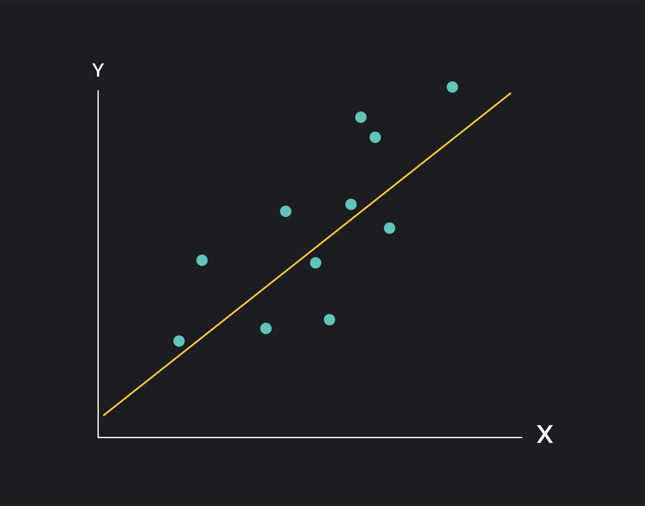
In linear regression, we estimate the relationship between the independent variable (X) and the dependent variable (Y) using a straight line. There are a few different ways to fit this line, but the most common method is called the Ordinary Least Squares Method (or OLS).

In OLS, you can find the regression line by minimizing the sum of squared errors. Here the errors—or residuals—are the vertical distances between each point on the scatter plot and the regression line. The regression coefficient on X tells you the slope of the regression line.

Regression Output Tables

We typically perform our regression calculations using statistical software like R or Stata. When we do this, we not only create scatter plots and lines but also create a regression output table like the one below. A regression output table is a table summarizing the regression line, the errors of your model, and the statistical significance of each parameter estimated by your model.

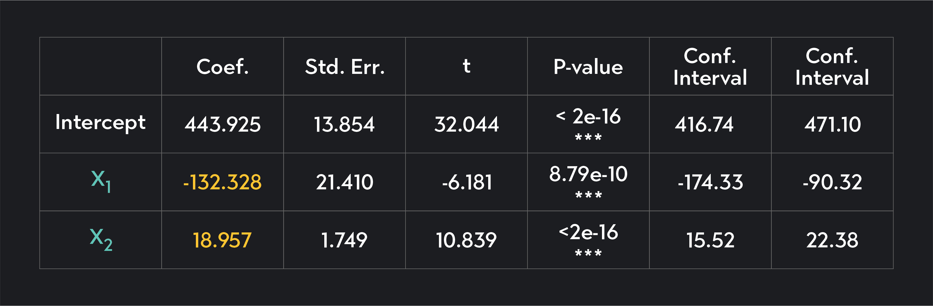
In the table here, the independent variables ($X_1$ and $X_2$) are listed in the first column of the table, and the coefficients on these variables are listed in the second column of the table in rows 3 and 4.

Regression Coefficient Interpretation

In linear regression, your regression coefficients will be constants that are either positive or negative. Here is how you can interpret the coefficients.

1. Non-Zero Coefficient

A non-zero regression coefficient indicates a relationship between the independent variable and the dependent variable.

2. Positive Coefficient

If the regression coefficient is positive, there is a positive relationship between the independent variable and the dependent variable. As X increases, Y tends to increase, and as X decreases, Y tends to decrease.

3. Negative Coefficient

If the regression coefficient is negative, there is a negative (or inverse) relationship between the independent variable and the dependent variable. As X increases, Y tends to decrease, and as X decreases, Y tends to increase.

Remember, your coefficients are only estimates. You’ll never know with certainty what the true parameters are, and what the exact relationship is between your variables.

In regression, you can estimate how much of the variation in your independent variable can be explained by a dependent variable by calculating $R^2$, and you can calculate how confident you can be in your estimates using tests of statistical significance.

How To Find Regression Coefficients

In a simple OLS linear regression of the form Y = $B_0 + B_1X$, you can find the regression coefficient $B_1$ using the following equation.

Chances are, however, that you will not be solving regression coefficients by hand. Instead, you’ll use software like Excel, R, or Stata to find your regression coefficients.

Regression Coefficients in Different Types of Regression Models

In this article, we’ve mainly discussed the simplest form of regression: a linear regression with one independent variable. As you continue to study statistics, you’ll encounter many more complex forms of regression. In these other regression models, the coefficients might take on slightly different forms and may need to be interpreted differently.

Here’s a list of some commonly used regression models.

Linear Regression

Linear regression is one of the most basic forms of regression. As you saw earlier, in linear regression, you find a line of best fit (a regression line) that minimizes the sum of squared errors. This line models the relationship between a dependent variable and an independent variable.

Logistic Regression (or Logit Regression)

We use a logistic regression when you want to study a binary outcome, and you are trying to estimate the likelihood of one of the two possible outcomes occurring. Logistic regression allows you to predict whether an outcome variable will be true or false, a win or a loss, heads or tails, 1 or 0, or any other binary set of outcomes.

In logistic regression, you interpret the regression coefficients differently than you would in a linear model. In linear regression, a coefficient of 2 means that as your independent variable increases by one unit, your dependent variable is expected to increase by 2 units. In logistic regression, a coefficient of 2 means that as your independent variable increases by one unit, the log odds of your dependent variable increase by 2.

Regression Models with Non-linear Terms

In a non-linear regression, you estimate the relationship between your variables using a curve rather than a line. For example, if we know that the relationship between Y and $X_1$ cannot simply be expressed by a line, but rather with a curve, we may want to include $X_1$, but also its quadratic version $X_1^2$. In this case, we will get two coefficients related to $X_1$1; one for $X_1$ and one for $X_1^2$. Something like this:

Here, we no longer can say that if $X_1$ changes by one unit, Y changes by 0.4 units since $X_1$ appears twice in the regression. Instead, the relationship between Y and $X_1$ is non-linear. If the level of $X_1$ is 1 and we increase it by 1 unit, then Y increases by (1.5 - 1) units.

However, if the level of $X_1$ is 2 and we increase it by 1 unit, then Y increases by (1.5 - 2). This is because the partial derivative of Y with respect to $X_1$ is no longer a constant and is 1.5 - 2 ✕ 0.5 $X_1$.

Ridge Regression

Ridge regression is a technique used in machine learning. Statisticians and data scientists use ridge regressions to adjust linear regressions to avoid overfitting the model to training data. In ridge regression, the parameters of the model (including the regression coefficients) are found by minimizing the sum of squared errors plus a value called the ridge regression penalty.

As a result of the adjustment, the dependent variables become less sensitive to changes in the independent variable. In other words, the coefficients in a ridge regression tend to be smaller in absolute value than the coefficients in an OLS regression.

Lasso Regression

Lasso regression is ‌similar to ridge regression. It is an adjustment method used with OLS to adjust for the risk of overfitting a model to training data. In a Lasso regression, you adjust your OLS regression line by a value known as the Lasso regression penalty. Similar to the Ridge regression, the lasso regression penalty shrinks the coefficients in the regression equation.

Explore Outlier's Award-Winning For-Credit Courses

Outlier (from the co-founder of MasterClass) has brought together some of the world's best instructors, game designers, and filmmakers to create the future of online college.

Check out these related courses: