Midpoint Formula: Definition, Uses & Examples

In This Article

1. What is the Midpoint Method Formula?

2. Midpoint Formula in Geometry

3. Midpoint Method in Economics

4. Interpreting the Result

5. A Price Elasticity Example

What is the Midpoint Method Formula?

In Economics, the midpoint method is a variation of the elasticity formula used to calculate a more accurate measure of how sensitive one economic variable is to percent changes in the value of another variable. Its name comes from the definition of a midpoint in geometry and, as we will see now, it has an important advantage for the calculations of elasticities.

Before we see what the midpoint formula is and how it works, we will have a look at the original definition in geometry and then use its economic application on the price elasticity of demand.

Midpoint Formula in Geometry

Imagine that you and a friend live in a grid city, where the locations of houses are given by points in the plane. For example, let’s say you live in (3,5) and your friend lives in (7,3). On New Year’s Eve, your friend and you have presents for each other and should meet so that you can exchange them. However, New Year’s Eve is a busy day and both of you would like to meet as close as possible to your respective homes so that you can save some time. Of course, a fair choice would be one where both of you must travel the same distance, and as you can already imagine, there are many possible places where this happens. So, which of all should you pick? Well, since New Year’s Eve is a busy day, you should pick the point where not only both of you travel the same distance, but this distance is also the shortest as possible. That place is called the midpoint and is quite easy to find.

A midpoint is a point lying in the segment line between two points which complies with being equidistant to each of the extreme points.

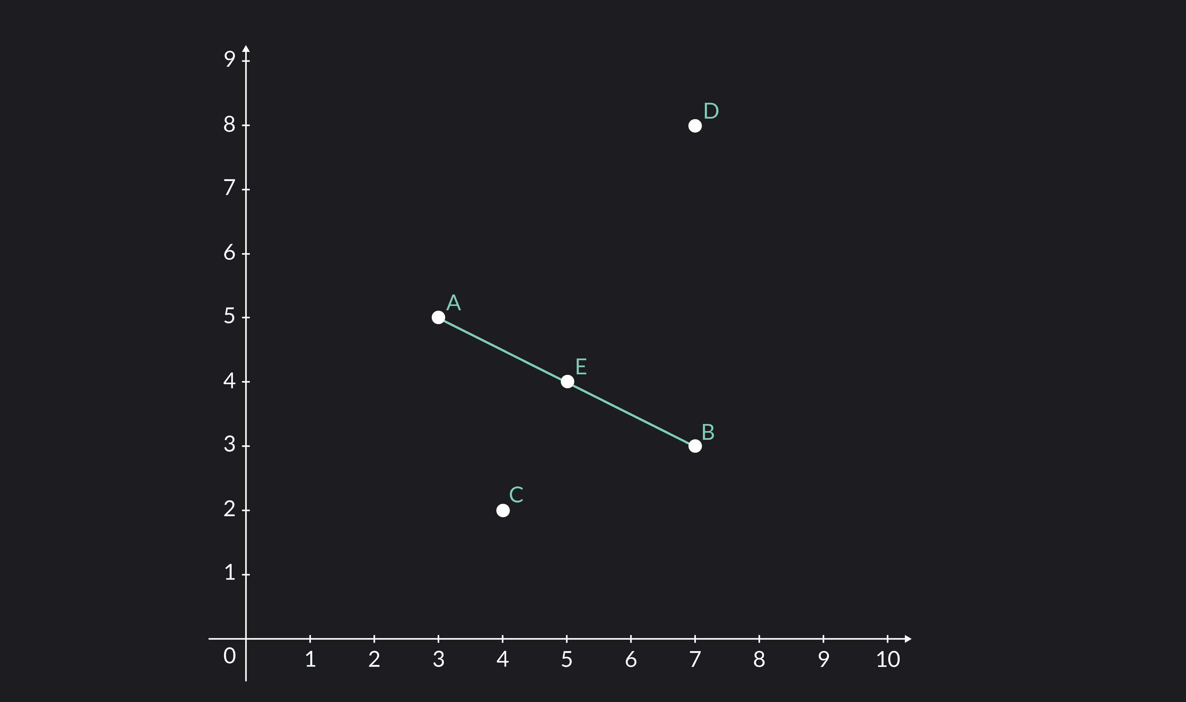
If you live in point A and your friend lives in point B, then points C, D, and E would be at the same distance from both of you; but point E is the closest one to both and as you can see, it lies in the middle of the segment between A and B.

Finding the midpoint is quite easy, the only thing you will need are the coordinates for both points and then use the following formula:

Back to our example, if you live in $(x_1, y_1) = (3, 5)$ and your friend lives in $(x_2, y_2) = (7, 3)$, then the midpoint where you should meet will be:

$\text{Midpoint} = (x_m, y_m) = (\frac{x_1 + x_2}{2}, \frac{y_1 + y_2}{2}) = (\frac{3 + 7}{2}, \frac{5 + 3}{2}) = (5, 4)$

Midpoint Method in Economics

Now, as we mentioned at the beginning, the midpoint formula happens to be useful to calculate elasticities. To make this easier to understand, let’s use it to calculate the price elasticity of demand in an example. But right before that, it would be useful to remember what an elasticity is.

Elasticity is a measurement of how percentage changes of one variable affect change in another variable.

Suppose we have the following demand function:

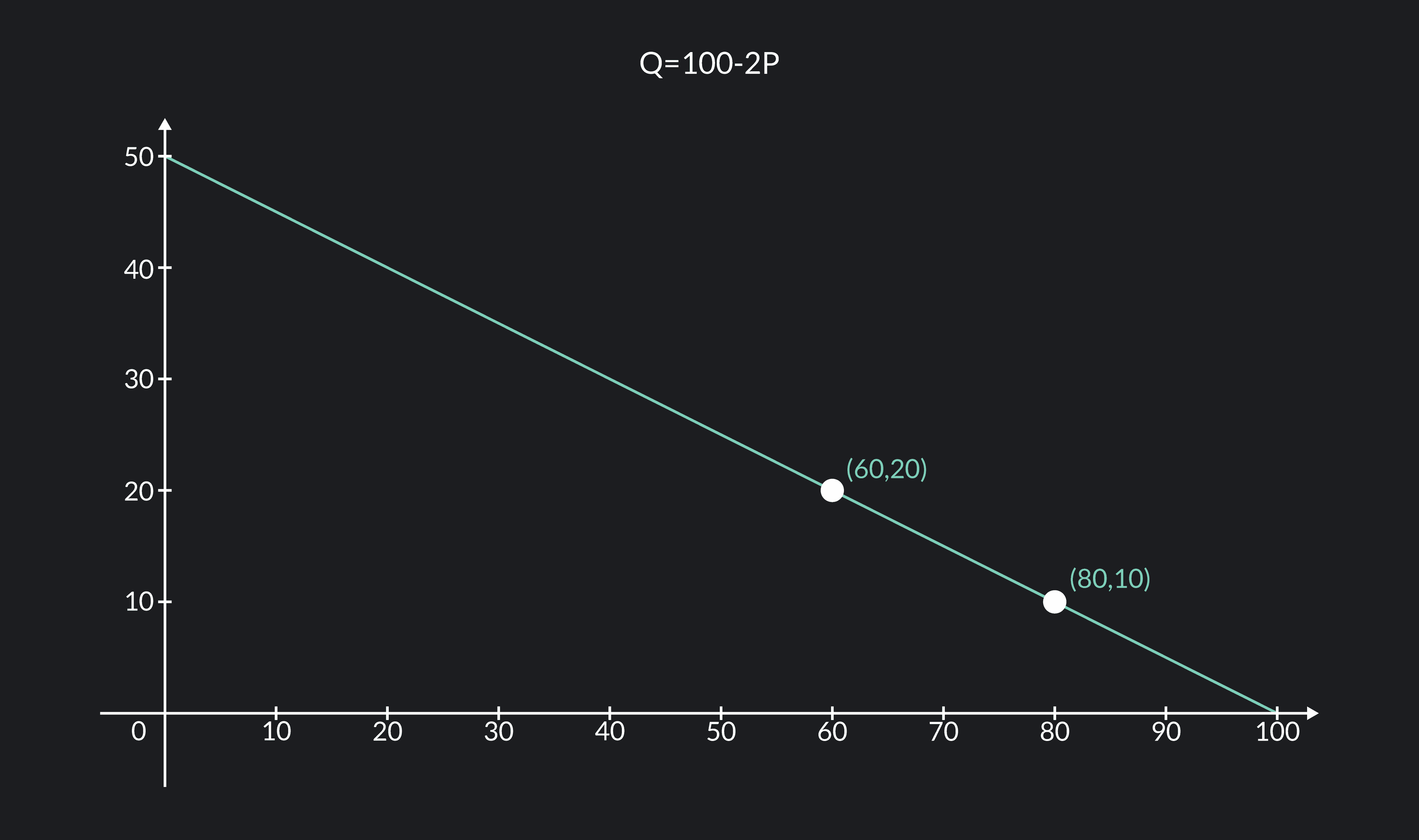
At given prices $P_1=10$ and $P_2 = 20$, the respective quantities demanded would be $Q_1 = 80$ and $Q_2 = 60$. We can use this information to calculate the price elasticity of demand—how the quantity demanded will change given a change in price.

In this example, the price shifted from $P_1 = 10$ to $P_2 = 20$, and the quantity then shifted from $Q_1 = 80$ to $Q_2 = 60$. The elasticity should be calculated by dividing the percentage change in quantity by the percentage change in price.

1. $\text{Percentage change in quantity } = \%\Delta Q = \frac{Q_2-Q_1}{Q_1}$

2. $\text{Percentage change in price } = \%\Delta P = \frac{P_2-P_1}{P_1}$

3. $\text{Price elasticity of demand } = \epsilon = \frac{\%\Delta Q}{\%\Delta P}$

So, by inputting the respective values, we can calculate the elasticity.

1. $\%\Delta Q = \frac{Q_2-Q_1}{Q_1} = \frac{60-80}{80} = -0.25$

2. $\%\Delta P = \frac{P_2-P_1}{P_1} = \frac{20-10}{10}$

3. $\epsilon = \frac{\%\Delta Q}{\%\Delta P} = \frac{-0.25}{1} = -0.25$

What would have happened if the shifts were the other way?

In this case the price would have shifted from $P_1 = 20$ to $P_2 = 10$, and in consequence the quantity would have shifted from $Q_1 = 60$ to $Q_2 = 80$. Intuitively, since the quantities and prices are the same but in an opposite direction, we would expect the elasticity to be the same.

1. $\%\Delta Q = \frac{Q_2-Q_1}{Q_1} = \frac{80-60}{60} \approx 0.3333$

2. $\%\Delta P = \frac{P_2-P_1}{P_1} = \frac{10-20}{10} = -0.5$

3. $\epsilon = \frac{\%\Delta Q}{\%\Delta P} = -\frac{0.3333}{0.5} \approx -0.6666$

What happened here? Well, it happens that it is not the same to shift the price from 10 to 20 (which would mean a 100% increase) than from 20 to 10 (which would mean a 50% reduction), and the same logic applies to the quantities. Therefore, since the percentage changes are different, then the calculation of the elasticity is affected. But remember, elasticity is a measure of how sensitive the quantity is to percentual changes in price. This kind of change should not be affected by the size of the change itself!

To solve this problem, we can use a new variation of the elasticity formula based on the midpoint formula that we have just understood above. Now, instead of measuring change related to the original value, we will measure it related to the average. For example, originally the percentage change in quantity was defined as:

Now, instead of using $Q_{1}$ as a reference in the denominator, we will use the $Q_{M}$ from the midpoint (which was basically the average of $Q_{1}$ and $Q_{2}$.

$\text{Percentage change in quantity (using the midpoint) } = \%\Delta Q = \frac{Q_2-Q_1}{Q_M} = \frac{Q_2 - Q_1}{ \frac{Q_1 + Q_2}{2}}$

And applying the same modification to the percentage change in price, we can define a new formula for the price elasticity of demand.

$\epsilon = \frac{\%\Delta Q}{\%\Delta P} = \frac{\frac{Q_2 - Q_1}{\frac{Q_1 + Q_2}{2}}}{\frac{P_2 - P_1}{\frac{P_1 + P_2}{2}}}$

Which can be written in a simpler way as:

$\epsilon = \frac{\%\Delta Q}{\%\Delta P} = \frac{(Q_2-Q_1)(P_1+P_2)}{(P_2-P_1)(Q_1+Q_2)}$

And this is the midpoint formula for the price elasticity of demand.

Now, we can use this formula to calculate the price elasticity of demand using the original information ($Q_{1}$,$P_{1}$)= (80,10) and ($Q_{2}$, $P_{2}$)= (60,20).

$\epsilon = \frac{\%\Delta Q}{\%\Delta P} = \frac{(Q_2-Q_1)(P_1+P_2)}{(P_2-P_1)(Q_1+Q_2)} = \frac{(60-80)(10+20)}{(20-10)(80+60)} \approx -0.4285$

And now, let’s use the formula again for the second scenario in which the shift happened in the opposite way ($Q_{1}$, $P_{1}$) = (60,20) and ($Q_{2}$, $P_{2}$) = (80,10).

$\epsilon = \frac{\%\Delta Q}{\%\Delta P} = \frac{(Q_2-Q_1)(P_1+P_2)}{(P_2-P_1)(Q_1+Q_2)} = \frac{(80-60)(20+10)}{(10-20)(60+80)} \approx -0.4285$

Now, you can see that our elasticity is not affected by the direction of the change!

Interpreting the Result

So far, we have used this formula to calculate a more accurate version of the price elasticity of demand. But how do we interpret this result?

It is really simple. The first thing to note is that the elasticity is already measured in percent points. So in this case, the ϵ = -0.42 means that for every 1% increase in the value of the price, the quantity demanded will decrease by 0.42%. In a more explicit example, if the price increases by 100%, the quantity demanded will decrease by 42%.

Since the percentage change in the quantity is smaller than the percentage change in the price, we say that we are in the inelastic part of the demand where quantity is not that sensitive to changes in prices.

The other case would have been observed if the elasticity were bigger than 1, that would have implied that for a 1% change in price, the % change in quantity would have been bigger than 1%, that is called the elastic part of demand where quantity is highly sensitive to changes in price.

A Price Elasticity Example

Suppose that we have a demand given by Q = 3000 - 25P. Let’s calculate the price elasticity of demand for two cases: first when we are on the elastic part of the demand (points A and B) and then when we are on the inelastic part of the demand (points C and D).

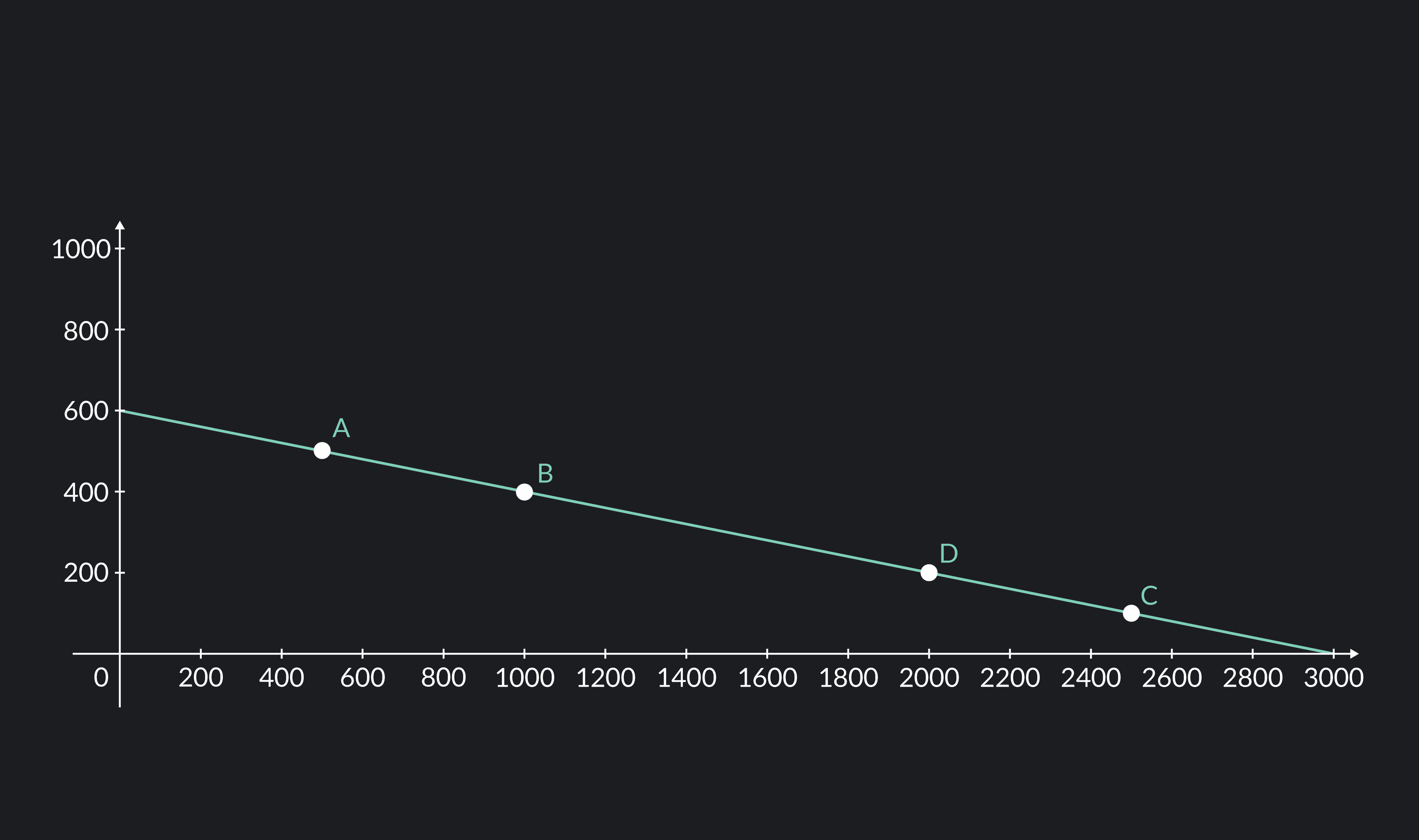
For the first case, we have ($Q_{A}$, $P_{A}$) = (500, 500) and ($Q_{B}$, $P_{B}$ = (1000, 400). We can use our formula to find the price elasticity of demand.

Note that it makes no difference which point you use as ($Q_{1}$, $P_{1}$) and which point you use as ($Q_{2}$, $P_{2}$) as long as you make sure to use them correctly—i.e. do not mix ($Q_{1}$, $P_{2}$) .

$\epsilon = \frac{\%\Delta Q}{\%\Delta P} = \frac{(Q_2-Q_1)(P_1+P_2)}{(P_2-P_1)(Q_1+Q_2)} = \frac{(1000-500)(500+400)}{(400-500)(500+1000)} = -3$

And we get ϵ = -3 which means that for a 1% increase in the price value, the quantity demanded will decrease 3%, note that since the % change in quantity is bigger than the % change in price, we are in the elastic part of the demand and quantity is highly sensitive to changes in price.

For the second case, we now have ($Q_{C}$, $P_{C}$) = (2500,100) and ($Q_{D}$, $P_{D}$) = (2000, 200). Once again we will use the midpoint formula to calculate the price elasticity of demand.

$\epsilon = \frac{\%\Delta Q}{\%\Delta P} = \frac{(Q_2-Q_1)(P_1+P_2)}{(P_2-P_1)(Q_1+Q_2)} = \frac{(2000-2500)(100+200)}{(200-100)(2500+2000)} \approx -0.33$

And our elasticity is ϵ = -0.33, so for a 1% increase in the price value, the quantity demanded will drop 0.33%. In contrast, a more visual way is if the price increases 100%, the quantity will decrease by 33%. Now we are on the inelastic part of demand where the quantity demanded by the consumers is not that sensitive to the changes in price.

Explore Outlier's Award-Winning For-Credit Courses

Outlier (from the co-founder of MasterClass) has brought together some of the world's best instructors, game designers, and filmmakers to create the future of online college.

Check out these related courses:

Intro to Microeconomics

Why small choices have big impact.

Explore course

Intro to Microeconomics

Why small choices have big impact.

Explore course

Intro to Macroeconomics

How money moves our world.

Explore course

Intro to Macroeconomics

How money moves our world.

Explore course

Principles of Economics

Economics in a nutshell.

Explore course

Principles of Economics

Economics in a nutshell.

Explore course

Intro to Statistics

How data describes our world.

Explore course

Intro to Statistics

How data describes our world.

Explore course