Derivative Formula: An Easy-To-Understand Guide

In This Article

1. What Is a Derivative Formula?

2. What Is a Derivative?

3. Elements of a Derivative

4. Key Derivative Formulas

5. Solving Derivatives Step by Step

6. Types of Derivatives

What Is a Derivative Formula?

Derivative formulas are equations that give quick solutions to common derivative problems. We refer to them as rules—like the power rule and the chain rule, to name a few.

More on these later.

These formulas come from the limit definition of the derivative, and they streamline the differentiation process. That’s why we can also call them differentiation formulas.

What Is a Derivative?

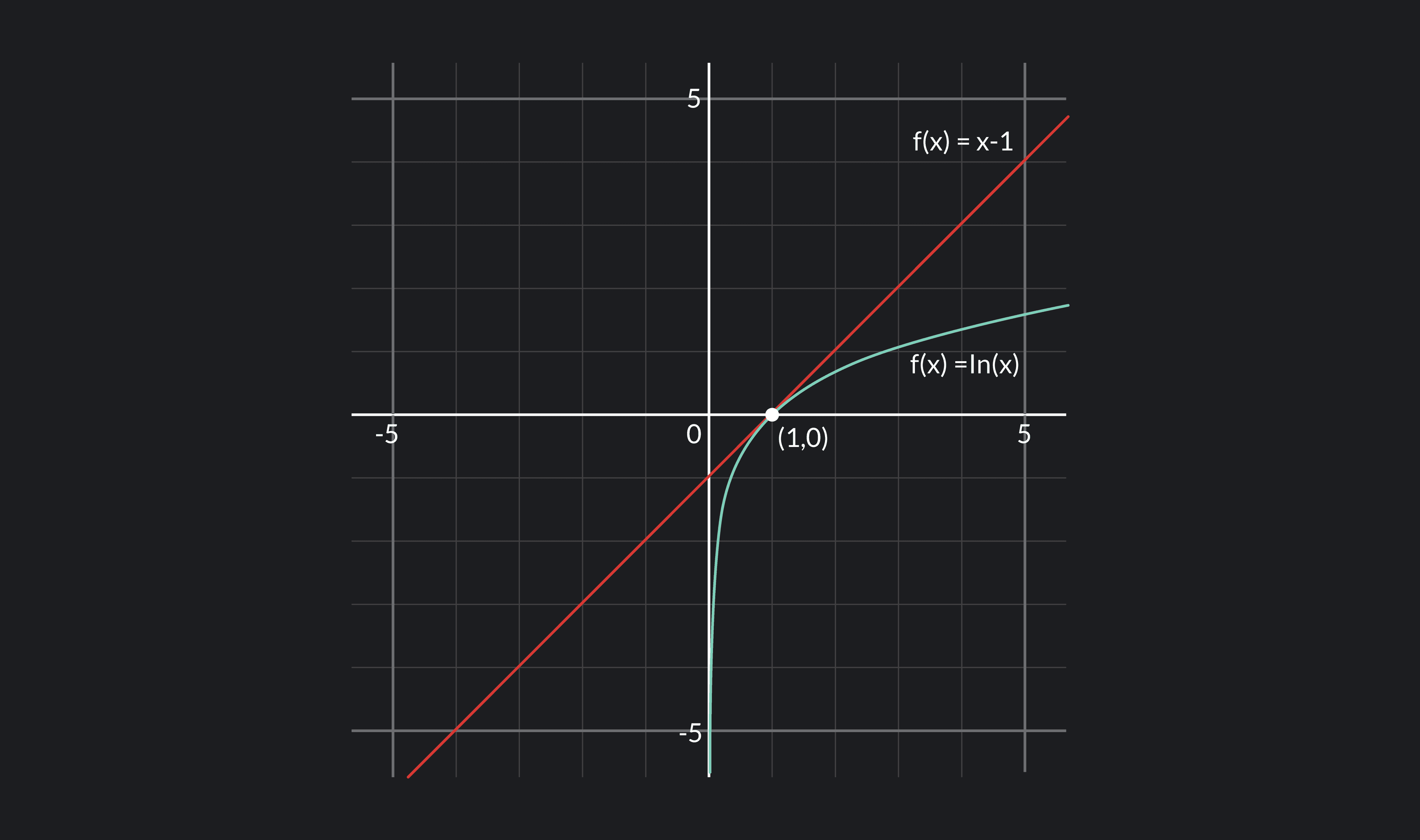
The derivative of a function at a point $x$ is equal to the slope of the tangent line at $x$.

This slope value represents the instantaneous rate of change at that point. Differentiation is the process of determining the derivative of a function.

For example, in the graph below, the function $f(x) = \ln{(x)}$ is in blue. The red line is $f(x) = x-1$, which is the line tangent to $f$ at $x = 1$. A tangent line to a point on a function is a line that just barely touches the function at that point. The slope of this tangent line $f(x) = x-1$ is $1$, which means that the derivative of $f(x) = \ln{(x)}$ is $1$ at $x = 1$.

We formally define derivatives using limits:

The above equation represents the limit of the average rate of change of $f$ over the interval $[x, x +\Delta{x}]$ as $\Delta{x}$ approaches 0. We also know the average rate of change of a function as the slope of the secant line.

In this notation, $\Delta{x}$ represents a small change in $x$. If this limit exists, then $L$ is the derivative.

Elements of a Derivative

The notation $f’(a)$ represents the derivative of a function $f$ at some point $a$. You might hear this notation read aloud as either “the derivative of $f$ evaluated at $a$” or “$f$ prime at $a$.”

The expressions $f’(x)$ and $\frac{dy}{dx}$ both represent the general derivative function of $f$. The latter notation is called Leibniz’s notation. By plugging any point $a$ into the resulting function $f’(x)$, we can determine the slope of the tangent line of $f$ at any point on the curve.

Key Derivative Formulas

It’s essential to know how to use the limit definition to calculate a derivative. However, the limit definition can be clunky to use. Usually, we rely upon the standard derivative formulas below to differentiate, instead of using the formal limit definition:

Constant Rule

$\frac{d}{dx}c = 0$

Power Rule

$\frac{d}{dx}(x^n) = nx^{n-1}$

Special Case of the Power Rule

This case is where $n$=1

$\frac d{dx}(x)=1$

Constant Multiple Rule

$\frac d{dx}(c\cdot f(x))=c\cdot f'(x)$

Chain Rule

$\frac{d}{dx}f(g(x)) = f’(g(x))g’(x)$

Product Rule

$\frac{d}{dx}[f(x) \cdot g(x)] = f’(x) \cdot g(x) + f(x)\cdot g’(x)$

Quotient Rule

$\frac{d}{dx}[\frac{f(x)}{g(x)}] = \frac{g(x)f’(x)-f(x)g’(x)}{(g(x))^2}$

Sum or Difference Rule

$\frac{d}{dx}[f(x) \pm g(x)] = f’(x) \pm g’(x)$

Trigonometry Rules

$\frac{d}{dx}(\sin{(x)}) = \cos{(x)}$

$\frac{d}{dx}(\cos{(x)}) = -\sin{(x)}$

$\frac{d}{dx}(\tan{(x)}) = \sec ^2 (x)$

Logarithmic Functions & Exponential Functions Rules

$\frac{d}{dx} (\ln{x}) = \frac{1}{x}$

$\frac{d}{dx}(e^x) = e^x$

Two game-changing derivative rules, according to Dr. Tim Chartier, are the product rule and quotient rule:

He also explains more differentiation formulas for finding with examples:

Solving Derivatives Step By Step

Now, we’ll discuss how to find derivatives. We can solve a derivative in two ways:

1. Using the formal limit derivative definition

2. Using the basic derivative formulas

Here are the steps to finding derivatives using the limit definition:

Step 1

Substitute your function into the limit definition of a derivative formula:

The hardest part of this step is the correct substitution of $x+h$ in the first term. You need to substitute $x$ with the expression $(x + \Delta{x})$ wherever $x$ appears in $f(x)$.

Step 2

Simplify.

Step 3

Evaluate the resulting limit.

Practice Example 1

For example, let’s find the derivative of the function $f(x) = 3x^2$.

Step 1 - Substitute

Let's sub in our function $f(x) = 3x^2$ into the limit definition of a derivative.

Step 2 - Simplify

We can do this by expanding the term $3(x + \Delta{x})^2$ and then combining like terms. Then we can divide by $\Delta{x}$ since $\Delta{x}$ is present in all terms of the numerator and denominator.

Step 3 - Evaluate

Now examine the limit as $\Delta{x}$ approaches 0. Polynomials are always continuous. To evaluate this limit, we can substitute $\Delta{x} = 0$ directly into the function we’re left with.

So, we’ve found that the derivative of $f(x) = 3x^2$ is $f’(x) = 6x$. This is the general derivative formula for any point on the curve of $f$.

To find the derivative at a single point, we can plug $x = a$ into $f’(x) = 6x$.

For example, we can say that:

• $f’(1) = 6(1) = 6$, which represents the slope of the tangent line at $x = 1$.

• $f’(5) = 6(5) = 30$, which represents the slope of the tangent line at $x = 5$.

• $f’(-60) = 6(-60) = -360$, which represents the slope of the tangent line at $x = -60$.

• $f’(0) = 6(0) = 0$, which represents the slope of the tangent line at $x = 0$.

Practice Example 2

We can also use the differentiation formulas to evaluate derivatives. For example, let’s find the derivative of $f(x) = 4x^4 + e^x$.

We can use the sum rule, which states that the derivative of a sum of functions is equal to the sum of their derivatives. We’ll also need to use the power rule for the $4x^4$ term, where our exponent is $n = 4$. Finally, we’ll use the exponential function rule for $e^x$, which tells us that $\frac{d}{dx}e^x = e^x$.

This gives us:

Practice Example 3

For a slightly trickier example, let’s find the derivative of $f(x) = \sin{(4x)}\cos{(2x)}$.

First, we’ll need the product rule. This says that the derivative of a product of functions is the sum of the first function times the derivative of the second, and the second function times the derivative of the first.

Along with the sine and cosine derivative rules, we’ll also need the chain rule, since we have a composition of functions using the sine and cosine functions.

The chain rule states that the derivative of a composition of functions is equal to the derivative of the outside function, multiplied by the derivative of the inside function.

This means that the derivative of $\sin{(4x)}$ is $4\cos{(4x)}$, and the derivative of $\cos{(2x)}$ is $-2\sin{(2x)}$.

Types of Derivatives

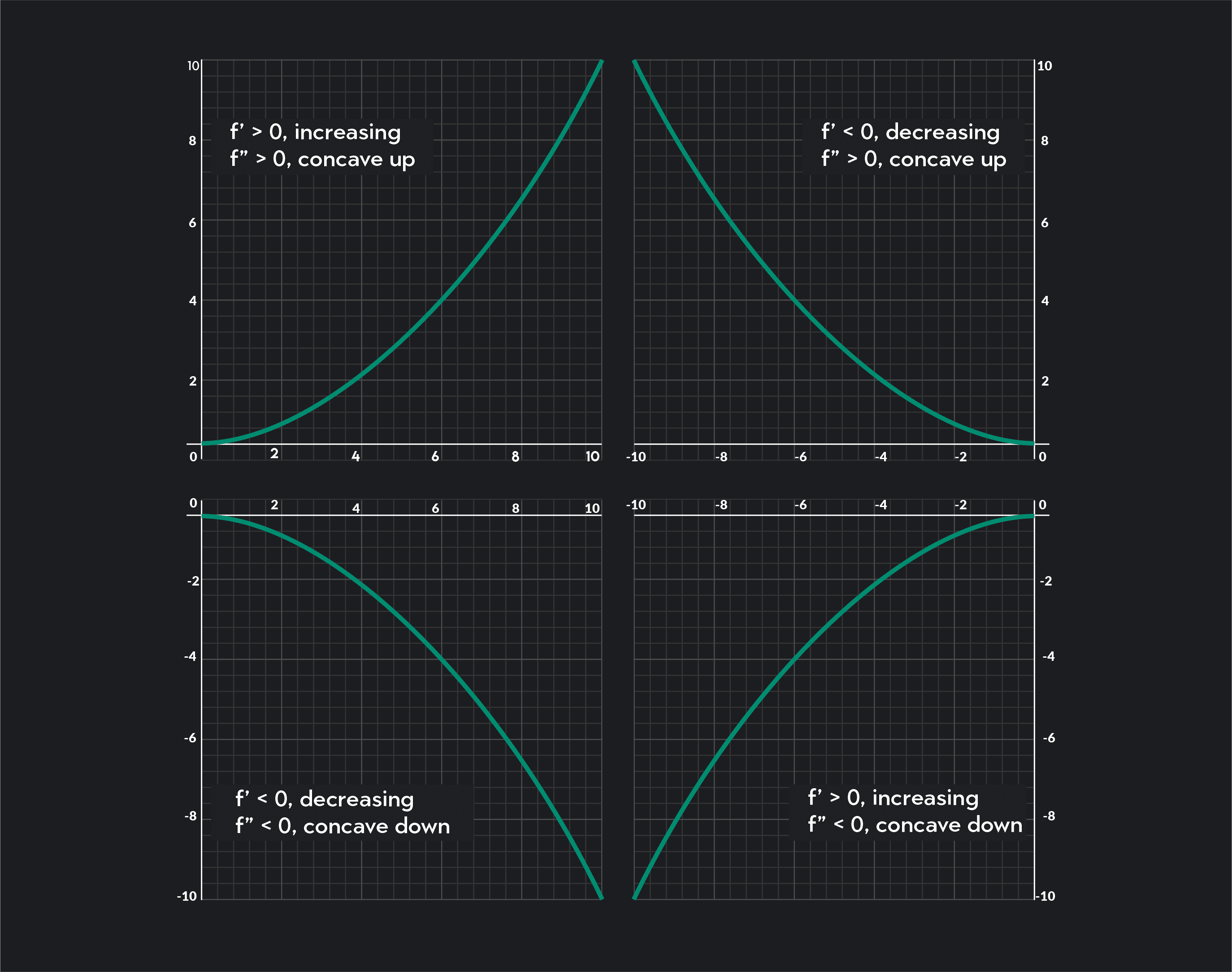
First and second derivatives provide different information about the behavior of a function.

We use the sign of the first derivative to determine if a function is increasing, decreasing, or constant on an interval $I$:

• If $f’(x) > 0$ for each $x$ on $I$, then $f$ is increasing on $I$.

• If f’(x) < 0 for each x on I, then f is decreasing on I.

• If $f’(x) = 0$ for each $x$ on $I$, then $f$ is constant on $I$.

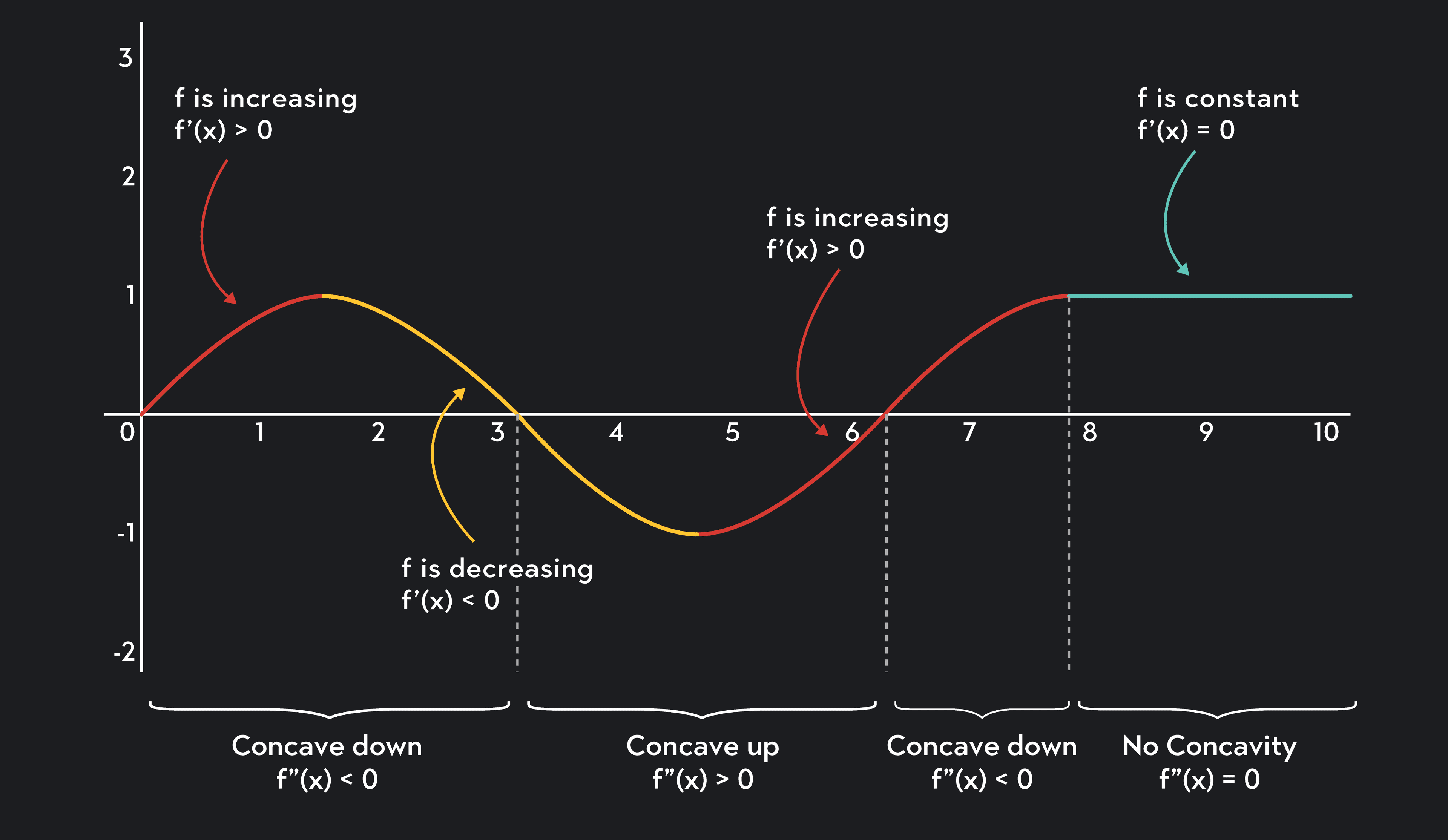
We find second derivatives by simply taking the derivative of the first derivative. Second derivatives inform us of the shape of a function. This characteristic is called concavity.

We use the sign of the second derivative to determine intervals of concavity:

• If $f’’(x) > 0$ for each $x$ on $I$, then $f$ is concave up on $I$.

• If f’’(x) < 0 for each x on I, then f is concave down on $I$.

• If $f’’(x) = 0$ for each $x$ on $I$, then $f$ has no concavity.

Dr. Hannah Fry discusses first and second derivative tests:

For more practice with differentiation and other skills in derivative calculus, Outlier’s calculus course is a rewarding resource. Here's why:

• Outlier offers accessible college classes at a fraction of the cost—80% less expensive than traditional college.

• Earn 3 college credits for every course you complete. Course accreditation is from the University of Pittsburgh, a top 60 school.

• Calculus courses are interactive and taught by world-renowned math professors, including Tim Chartier of Davidson College, Hannah Fry of University College London, and John Urschel of MIT.

• Course resources include question sets, quizzes, and an active-learning based digital textbook. You’ll also have access to free tutors and a study group.

• Transferring credits is easy.

• If you do the work and don’t pass, you’ll receive a full refund.

• Exam windows are flexible, and lectures are viewable on demand, anywhere.

Explore Outlier's Award-Winning For-Credit Courses

Outlier (from the co-founder of MasterClass) has brought together some of the world's best instructors, game designers, and filmmakers to create the future of online college.

Check out these related courses:

Calculus I

Watch trailer

Explore course

Calculus I

The mathematics of change.

Watch trailer

Explore course

Intro to Statistics

Watch trailer

Explore course

Intro to Statistics

How data describes our world.

Watch trailer

Explore course

Intro to Microeconomics

Watch trailer

Explore course

Intro to Microeconomics

Why small choices have big impact.

Watch trailer

Explore course