In This Article
What Does Multivariable Mean?
How to Solve Multivariable Calculus
Basic vs. Advanced Multivariable Calculus
Applications of Multivariable Calculus
What Does Multivariable Mean?
So far, our study of calculus has been limited to functions of a single variable. Multivariable calculus studies functions with two or more variables. Functions that take two or more input variables are called “multivariate.” These functions depend on two or more input variables to produce an output.
For example,
f(x,y)=x2+y is a multivariate function.
How to Solve Multivariable Calculus
How can we calculate derivatives in multivariable calculus? The derivative or rate of change in multivariable calculus is called the gradient. The gradient of a function f is computed by collecting the function’s partial derivatives into a vector. The gradient is one of the most fundamental differential operators in vector calculus. Vector calculus is an important component of multivariable calculus that is concerned with the study of vector fields.
The notation for the gradient vector is ∇f. For a function with two variables, the gradient looks like this:
∇f(x,y)=⟨∂x∂f(x,y),∂y∂f(x,y)⟩ In this notation, ∂x∂f(x,y) is the partial derivative of f with respect to x. We obtain ∂x∂f(x,y) by treating x as a variable and y as a constant, and then differentiating.
Similarly, ∂y∂f(x,y) is the partial derivative of f with respect to y. We obtain ∂y∂f(x,y) by treating y as a variable and x as a constant, and then differentiating.
Partial derivatives help us to understand the behavior of a multivariate function when one variable changes while the rest are held constant.
Partial Derivative Example
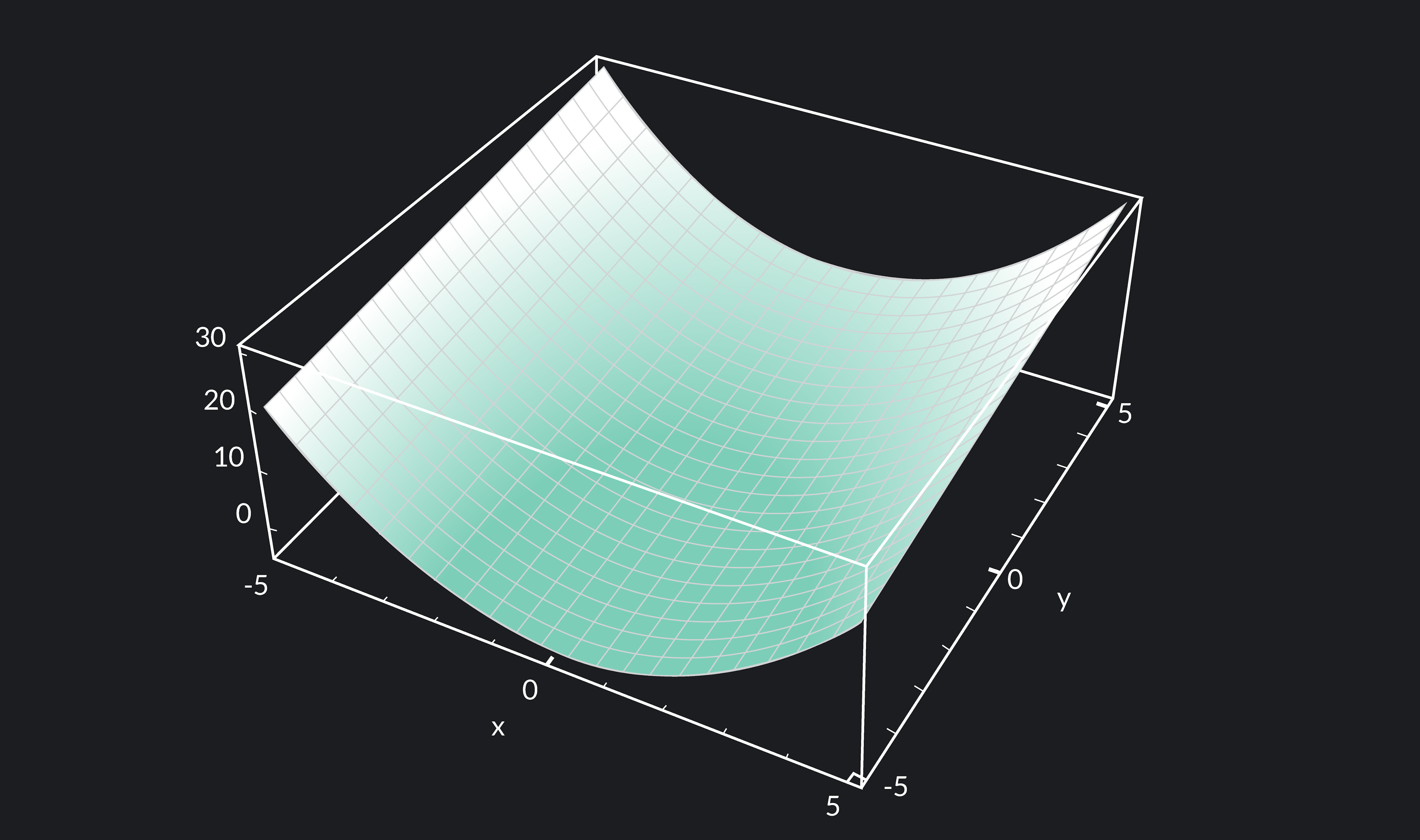
Let’s do one example together. We’ll calculate the gradient of f(x,y)=x2+y at (1,2). The plot of f(x,y)=x2+y can be seen below.
First, we’ll calculate ∂x∂f(x,y), the partial derivative of f with respect to x. Treating y as a constant and differentiating normally, we find that ∂x∂f(x,y)=2x. Remember that the derivative of any constant is zero.
Next, we’ll calculate ∂y∂f(x,y), the partial derivative of f with respect to y. Treating x as a constant and differentiating normally, we find that ∂y∂f(x,y)=1.
Collecting these components into a vector, we find that ∇f(x,y)=⟨2x,1⟩.
Plugging in our point (1, 2), we find that ∇f(1,2)=⟨2,1⟩. Thus, the gradient of f at (1, 2) is ⟨2,1⟩.
What insight does the gradient give us? Recall that the gradient is a vector. Vectors have both a magnitude and a direction. The gradient of a function f points in the direction of greatest increase of f. The direction of greatest increase can also be thought of as the direction of steepest ascent, the direction of the greatest rate of change, and the direction where f increases the fastest.
Basic vs. Advanced Multivariable Calculus
Both basic and advanced multivariable calculus concepts will involve the study of multivariable integration and multivariable differentiation. What are some of the most basic concepts in basic multivariable calculus?
Below is a list of 4 fundamental multivariable calculus concepts.
1. Partial Derivatives
Partial derivatives show us how a multivariate function behaves when we change just one variable while the rest are held constant. In multivariable calculus, partial derivatives are used to calculate the gradient.
2. Gradient Vectors
The gradient vector ∇f(x,y) is the collection of partial derivatives of f. The gradient points in the direction of the greatest increase of f. In the same vein, the opposite direction −∇f(x,y) is the direction of the greatest decrease of f.
3. Double Integrals
Recall that the definite integral ∫abf(x) is used to calculate the area under a curve. Similarly, the double integral ∫R∫f(x,y)dydx may be used to calculate the volume under a surface, where R is the region of integration.
Any study of double integrals will cover Fubini’s Theorem, which states that we can evaluate double integrals using iterated integrals and that the order of integration does not matter in its computation. We can visualize iterated integrals below in Fubini’s Theorem.
∫R∫f(x,y)dydx=∫ab∫cdf(x,y)dydx=∫cd∫abf(x,y)dxdy (You can also review our beginner’s guide to integrals if needed).
4. Relative Maxima and Minima
Relative maxima and minima are “peaks” on a multivariate function’s graph. At a relative maximum, moving in any direction will decrease the value of the function. At a relative minimum, moving in any direction will increase the value of the function. You can visualize relative maxima and minima in multivariable calculus as stalagmites and stalactites in a cave. These points are called extrema, and their gradients are 0.
Critical points are points on a function’s graph where the derivative is either zero or undefined. Not all critical points of a multivariate function are relative extrema, but the relative extrema of a multivariate function are always critical points. Much of calculus is concerned with finding and classifying critical points.
What kind of advanced concepts can you expect to cover in a multivariable calculus course?
Below is a list of 6 advanced multivariable calculus concepts.
Second-Order Partial Derivatives and Higher-Order Partial Derivatives
To compute second-order partial derivatives, we calculate the partial derivatives of the partial derivatives of a function. These higher-order derivatives can be used to check the concavity and extrema of a multivariate function.
Triple Integrals
While double integrals integrate over a two-dimensional region, triple integrals integrate over a three-dimensional region.
The Multivariable Chain Rule
The multivariable chain rule is derived from the chain rule in single-variable calculus. Suppose that we have two multivariable functions, x=g(u,v) and y=h(u,v). Let z=f(x,y)=f(g(u,v)),h(u,v)).
Then the multivariable chain rule states that the partial derivatives of f(g(u,v)),h(u,v)) at (u,v) are given by
∂u∂z=∂x∂z∂u∂x+∂y∂z∂u∂y and ∂v∂z=∂x∂z∂v∂x+∂y∂z∂v∂y
Four Critical Theorems
The following four theorems are some of the most important theorems in multivariable calculus:
All four theorems are concerned with multivariable integration. While they require more context than is appropriate for this brief overview, they are exciting theorems to look forward to in your study of multivariable calculus.
The Jacobian Determinant
The Jacobian matrix is the matrix of all the first-order partial derivatives of a function. When the Jacobian matrix is square, meaning that it has the same number of rows and columns, then its determinant is called the Jacobian determinant. The Jacobian determinant at a given point provides very valuable information about the function’s behavior and invertibility near that point.
More Vector Calculus and Matrices
Many multivariable calculus or Calculus 3 courses include a vector calculus component.
Vector calculus is a subdivision of calculus underneath the broader umbrella category of multivariable calculus and involves:
Applications of Multivariable Calculus
Many phenomena require more than one input variable to construct a sufficient mathematical model. Because of this, multivariable calculus is useful in many disciplines. Here are four examples of real-world applications of multivariable calculus.
Example 1
Multivariable calculus is useful in business and finance. For example, a company’s profit depends on multiple independent variables, such as pricing, sales, the cost of materials, and overhead costs. Multivariable calculus is necessary to calculate profit maximization.
Example 2
Multivariable calculus is essential to electrical engineering. Maxwell’s equations, a set of four partial differential equations, make up the backbone of electromagnetism. These equations, which explain the behavior of the different frequency ranges in the electromagnetic spectrum, encouraged the development of vector calculus in physics. Multivariable calculus is fundamental to understanding the behavior of electric fields and optimizing new electric technologies.
Example 3
We use multivariable calculus in graphics, programming, animation, and game development to model 3D worlds. For example, multivariable calculus is handy for modeling the movement of different curves and surfaces and developing lighting models.
Example 4
Most algorithms in machine learning depend on multiple variables. Many algorithms themselves rely on multivariable calculus concepts. For example, an algorithm called gradient descent is an optimization algorithm used to minimize a cost function.
Explore Outlier's Award-Winning For-Credit Courses
Outlier (from the co-founder of MasterClass) has brought together some of the world's best instructors, game designers, and filmmakers to create the future of online college.
Check out these related courses: