Methods of Integration: Techniques & Examples

In This Article

1. What Is Integration in Calculus?

2. 9 Essential Integration Rules

3. 4 Types of Integration Methods

4. More Calculus Practice

What Is Integration in Calculus?

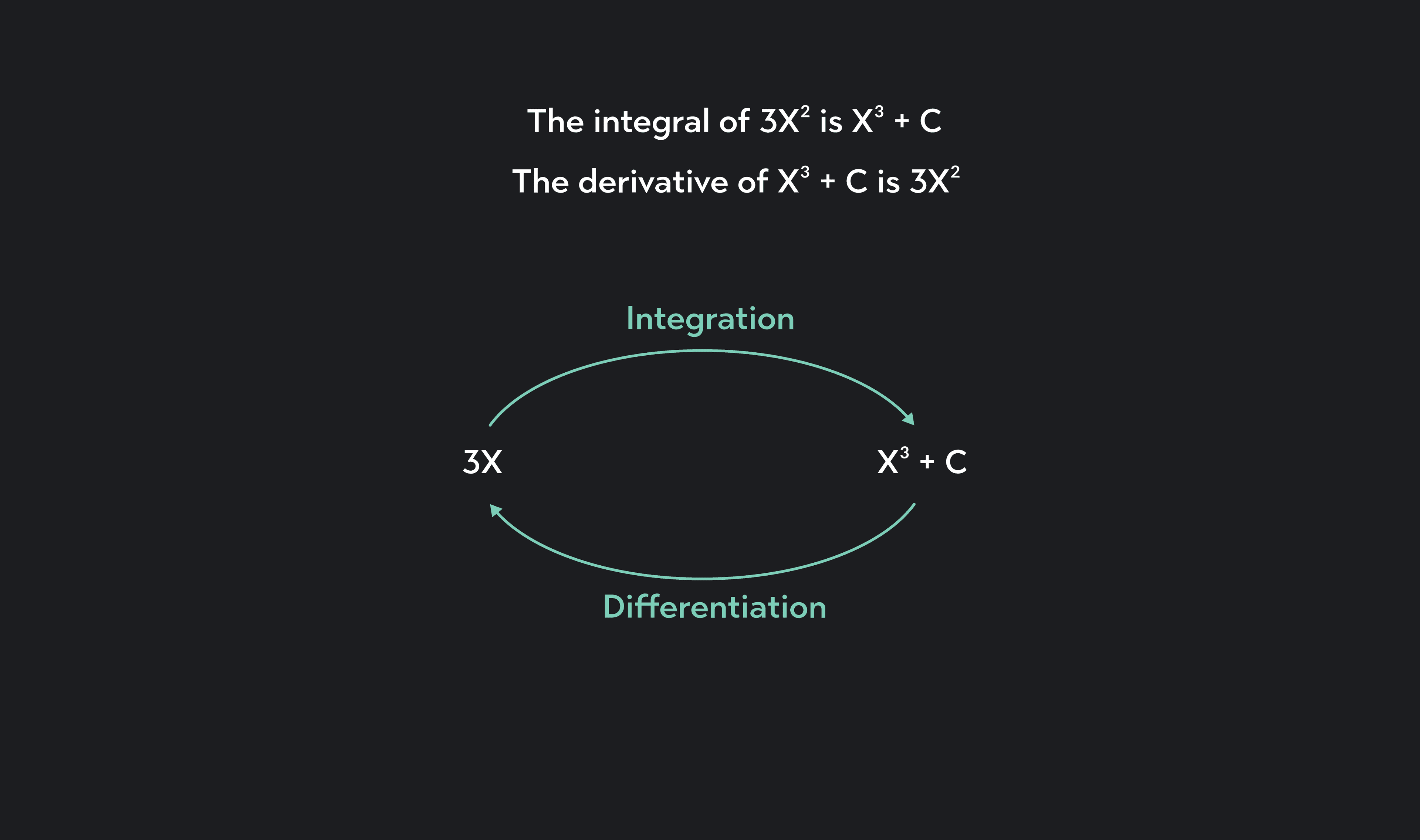
Differentiation finds the instantaneous rate of change of a function. Integration finds the reverse of a derivative, called the antiderivative. Integration can be conceptualized as the reverse process of differentiation.

Together, differentiation and integration constitute the fundamental operations of calculus. Their relationship is explained by the fundamental theorem of calculus.

There are two types of integrals: indefinite integrals and definite integrals. Indefinite integrals find antiderivative functions. Definite integrals calculate areas under the curve on a specific interval.

The notation for an indefinite integral is given below:

An indefinite integral finds the antiderivatives of $f(x)$, which are usually denoted by $F(x)$. Taking the derivative of $F(x)$ outputs back $f(x)$, which explains why $F$ is called an antiderivative function. For this reason, integration is also sometimes referred to as anti-differentiation:

For example,

The symbol $\int$ is called the integral sign, and $f(x)$ is called the integrand. The capital letter $C$ is called the constant of integration. $C$ is used to represent any constant value.

Remember that taking the derivative of the antiderivative of $f(x)$ gives back $f(x)$ itself. No matter what constant value $C$ holds, the derivative of $C$ will always be zero. So, when we take the derivative of $F(x) + C$, we always get back $f(x)$ alone. Thus $C$ can take any value, and for this reason, the notation $F(x) + C$ represents an infinitely large family of all antiderivatives of the function $f$.

The first fundamental theorem of calculus guarantees the relationship described earlier. If $f$ is a continuous function on an interval containing $a$, then we can define $F$ by:

Then $F’(x) = f(x)$ and so $F(x)$ is an antiderivative of $f(x)$:

Now, let’s review the notation for a definite integral:

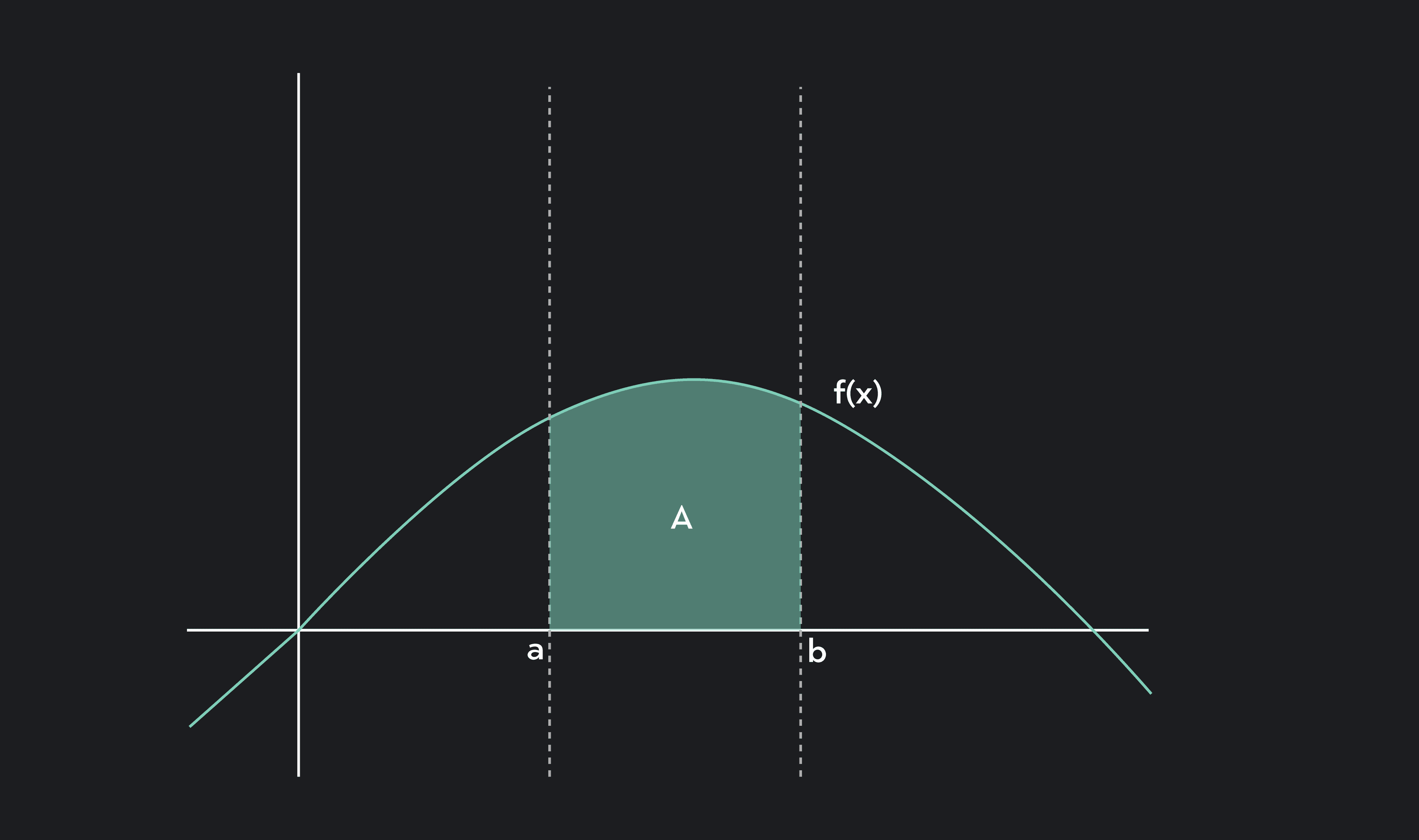
$A$ represents the area under the curve on $[a, b]$. To approximate this area, we could create $n$ rectangles of equal width that approximate the curve, and then take the sum of their areas. This approximation is called a Riemann sum. However, this sum either overestimates or underestimates the area under the curve.

By taking the limit of the Riemann sum as the number of subdivisions $n$ approaches infinity, we obtain the precise area under the curve. This defines a definite integral.

The second fundamental theorem of calculus clarifies the relationship between the integral and the antiderivative function. This theorem tells us that we can find the definite integral of a function on $[a, b]$ by taking the difference between the indefinite integral of the function evaluated at $a$ and the indefinite integral of the function evaluated at $b$.

For a good overview of this theorem, Dr. Hannah Fry shares what this theorem actually means, how it’s calculated, and what it can further allow us to do:

9 Essential Integration Rules

Now that we’ve defined integrals, it’s important to know how to evaluate them. These integration formulas are used in every method of integration, so it’s a good idea to memorize them.

1. Sum Rule

$\int [f(x) + g(x)]\,dx = \int f(x)\,dx + \int g(x)\,dx$

2. Difference Rule

$\int [f(x) - g(x)]\,dx = \int f(x)\,dx - \int g(x)\,dx$

3. Constant Multiplier Rule

$\int kf(x)\,dx = k\int f(x)\,dx$ for some constant $k$

4. Power Rule

Power Rule: $\int x^n\,dx = \frac{x^{n+1}}{n+1} + C$ for some real number $n$

5. Constant Rule

$\int a\,dx = ax + C$ for some constant $a$

6. Reciprocal Rules

• $\int \frac{1}{x}\,dx = \int x^{-1}\,dx = \ln{|x|} + C$

• $\int\frac{1}{ax+b}\,dx = \frac{1}{a} \ln{(ax+b)} + C$

Dr. Tim Chartier covers core differentiation rules and examples of how to use them:

7. Exponential Functions & Logarithmic Functions Rules

• $\int e^x\,dx = e^x + C$

• $\int a^x\,dx = \frac{a^x}{\ln{(a)}} + C$, for any positive real number $a$

• $\int \ln{(x)}\,dx = x\ln{(x)}-x + C$

8. Trigonometric Functions & Inverse Trigonometric Functions Rules

For these rules, assume that $x$ is in radians.

• $\int \sin{x}\,dx = -\cos{x} + C$

• $\int \cos{x}\,dx = \sin{x} + C$

• $\int \sec ^2 x\,dx = \tan{x} + C$

• $\int \csc ^2 x\,dx = -\cot{x} + C$

• $\int \sec{x}\tan{x}\,dx = \sec{x} + C$

• $\int \csc{x}\cot{x}\,dx = -\csc{x} + C$

• $\int \frac{dx}{\sqrt{1-x^2}}=\sin ^{-1}x + C$

• $\int \frac{-dx}{\sqrt{1-x^2}}=\cos ^{-1}x + C$

• $\int \frac{dx}{1+x^2}=\tan ^{-1}x + C$

• $\int \sin{(ax)}\,dx = \frac{-\cos{(ax)}}{a}+C$ for some real number $a$

• $\int \cos{(ax)}\,dx = \frac{\sin{(ax)}}{a}+C$ for some real number $a$

9. Absolute Value Rule

$\int |x|\,dx = \frac{x |x|}{2} + C$

4 Types of Integration Methods

We’ll discuss four essential techniques of integration:

1. Integration by u-substitution

2. Integration by parts

3. Integration by partial fractions

4. Integration using trigonometric identities

Integration by U-Substitution

U-substitution is used to integrate composite functions. U-Substitution reverses the chain rule. For this reason, u-substitution is also called the reverse chain rule. To use u-substitution, we rewrite our integral in terms of $u$ and $du$:

We can use the four steps below for integration by substitution:

1. Pick one part of the integrand to represent $u$. Usually, $u$ is equal to $g(x)$, the inner function of the composite function.

2. Differentiate $u$ to find $du$. If necessary, rearrange the problem algebraically so that $du$ perfectly matches what’s left inside the integral.

3. Substitute $u$ and $du$ into the integrand, and integrate. If taking a definite integral, redefine your limits of integration in terms of $u$.

4. If taking an indefinite integral, substitute the original values back into the resulting function and add the constant of integration to your final answer. If taking a definite integral, simply evaluate using the new limits in terms of $u$.

For example, let’s evaluate $\int \frac{[\ln{(x)}]^2}{x}dx$. Let $u = \ln{(x)}$, so that $du = \frac{1}{x}dx$. Substituting $u$ and $du$ into the integrand, we get:

Integration by Parts

Integration by parts is used to take the integral of a product of functions. Integration by parts uses the formula below, which is derived directly from the product rule for derivatives:

We can use the four steps below to integrate by parts:

1. Choose $u$ and $dv$ to separate the given function into a product of functions. Generally, $u$ is the term that’s easiest to differentiate, and $dv$ is the term that’s easiest to integrate.

2. Differentiate $u$ to find $du$, and integrate $dv$ to find $v$.

3. Plug $u$, $v$, and $du$ into the integration by parts formula.

4. Solve and simplify where needed.

For example, let’s evaluate $\int x\sin(x)dx$. Let $u=x$ and $dv=\sin(x)dx$. Differentiating $u$, we find that $du = 1dx$. Integrating $dv$, we find that $v = - \cos(x)$. Plugging $u=x$, $v = - \cos(x)$, $du = 1dx$, and $dv=\sin(x)dx$ into the integration by parts formula, we get:

The acronym LIATE can help you decide which term to designate as $u$. LIATE stands for:

• Logarithmic functions

• Inverse trigonometric functions

• Algebraic functions

• Trigonometric functions

• Exponential functions

Function types that sit the highest on this list should be prioritized as $u$.

Integration by Partial Fractions

Integration by partial fractions is used to integrate rational functions. A rational function is an algebraic fraction where both the numerator and denominator are polynomials.

We can use the nine steps below to integrate by partial fractions:

1. Factor the denominator of the function.

2. Decompose the function into a sum of its parts by assigning an unknown variable to each term of the denominator.

3. Combine all terms into one by finding the common denominator, making sure you multiply each numerator appropriately.

4. Multiply out the numerator.

5. Set up an equation that equates the $x$ terms of the original function’s numerator with the $x$ terms in your new equation’s numerator.

6. Set up a second equation that equates the constant terms of the original function’s numerator with the constant terms in your new numerator.

7. Solve for the unknown variables.

8. Plug your solved variables into Step 2.

9. Integrate using the reciprocal rules.

For example, let’s evaluate $\int \frac{x+4}{x^2+x-12}dx$. First, we’ll factor the denominator. Then, we can proceed with steps 2 through 4.

Now,

Our next step is to solve for $A$ and $B$ using steps 5 through 7. Our first equation is $Ax + Bx = x$. We can simplify this equation to $A+B=1$. Our second equation is $-3A+4B=4$. This gives us a system of equations, which outputs that $A = 0$ and $B = 1$.

Using steps 8 through 9, we have:

This technique is also called partial fraction decomposition.

Integration Using Trigonometric Identities

Here are some of the most important trigonometric identities to know:

Pythagorean Identities

• $\sin^2x + \cos^2x = 1$

• $\sec^2 x - \tan^2 x = 1$

• $\csc^2 x - \cot^2 x = 1$

Quotient and Reciprocal Identities

• $\tan x = \frac{\sin x}{\cos x}$

• $\cot x = \frac{\cos x}{\sin x}$

• $\sin x = \frac{1}{\csc x}$

• $\cos x = \frac{1}{\sec x}$

• $\tan x = \frac{1}{\cot x}$

• $\csc x = \frac{1}{\sin x}$

• $\sec x = \frac{1}{\cos x}$

• $\cot x = \frac{1}{\tan x}$

Double Angle Identities

• $\sin{(2x)} = 2 \sin x \cos x$

• $\cos{(2x)} = \cos^2 x - \sin^2 x = 2\cos^2 x - 1 = 1 - 2\sin^2 x$

• $\tan{(2x)} = \frac{2 \tan x}{1 - \tan^2 x}$

You can use trigonometric substitution with the above identities to help solve tricky integrals involving trigonometric functions.

For example, let’s evaluate \int_0^{\pi} \sin^2 x \, \dx. We’ll first use the double angle identity \cos{(2x)} = 1 - 2\sin^2 x, rearranging it to find that \sin^2 x = \frac{1}{2}(1-\cos{(2x)}. Then, we’ll use the trigonometric integral rule for cosine with an inner coefficient and integrate as usual.

More Calculus Practice

With the world’s most engaging instructors, Outlier’s calculus course offers a cinematic and immersive curriculum that prioritizes student success. It’s an affordable route to improving your mastery of integral calculus.

• Outlier offers accessible college classes at a fraction of the cost — 80% less expensive than traditional college!

• Earn 3 college credits towards your degree for every course you complete. Credits are received from the University of Pittsburgh, a top-60 school.

• Calculus courses are interactive and taught by world-renowned math professors, including Tim Chartier of Davidson College, Hannah Fry of University College London, and John Urschel of MIT.

• Course resources include question sets, quizzes, and an active-learning-based digital textbook. You’ll also have access to free tutors and a study group.

• Transferring credits is easy.

• If you do the work and don’t pass, you’ll receive a full refund.

• Exam windows are flexible, and lectures are viewable on-demand, anywhere.

Explore Outlier's Award-Winning For-Credit Courses

Outlier (from the co-founder of MasterClass) has brought together some of the world's best instructors, game designers, and filmmakers to create the future of online college.

Check out these related courses:

Calculus I

The mathematics of change.

Explore course

Calculus I

The mathematics of change.

Explore course

Intro to Statistics

How data describes our world.

Explore course

Intro to Statistics

How data describes our world.

Explore course

Intro to Microeconomics

Why small choices have big impact.

Explore course

Intro to Microeconomics

Why small choices have big impact.

Explore course