Derivative Basics - Representations Explained

In This Article

1. What Does the Derivative Represent?

2. 3 Steps on How To Calculate Derivatives

3. Derivatives and Rates of Change

4. Derivatives and Slopes of Tangent Lines

5. Derivatives and Velocity

What Does the Derivative Represent?

Derivatives measure rates of change. More specifically, derivatives are concerned with instantaneous rates of change. The instantaneous rate of change of a function at $x = a$ is equal to the slope of the tangent line at $x = a$.

What is a derivative exactly? We can formally define the derivative of a function using limits:

The limit given above defines a function $f’(x)$, which is called the derivative. This function $f’(x)$ allows us to assign some value $f’(a)$ to each number $a$ in the domain of $y = f(x)$:

If this limit exists at $x = a$, then $L$ is the derivative of the function at $x = a$.

If this limit does not exist at $x = a$, then there is no tangent, and so the function is not differentiable at $a$.

If a function is differentiable at every point in its domain, then we consider it a differentiable function.

3 Steps on How To Calculate Derivatives

Below are 3 steps to calculating derivatives using the limit definition of a derivative:

1. Substitute

Substitute your function into the limit definition of a derivative formula. To do this, replace $x$ with the expression $(x + \Delta{x})$ wherever $x$ appears in $f(x)$. Be cautious here and remember that $f(x + h) \neq f(x) + f(h)$.

2. Simplify

3. Evaluate

Evaluate the resulting limit.

The symbol $\Delta{x}$ represents a small value that $x$ changes by. By evaluating the limit as $\Delta{x}$ approaches zero, we obtain an instantaneous rate of change.

Alternatively, you might also see $f’(x)$ expressed by using the substitution $b = x + h$:

Similarly, $f’(a)$ will use the substitution $b = a + h$:

The derivative $f’(x)$ represents two things. First, $f’(x)$ represents the instantaneous rate of change of $y = f(x)$ with respect to $x$, for all values of $x$ where the limit exists. Second, $f’(x)$ represents the slope of the curve of $f(x)$ at any point in its domain.

In the next sections, we’ll go into more detail about the meaning of rates of change and tangent lines, and their relationship with derivatives.

Derivatives and Rates of Change

Rates of change describe the change that occurs in one variable as another variable changes. More specifically, rates of change represent the change in the dependent variable as the independent variable changes.

For any function $f$, the average rate of change over the interval $[a, b]$ is given by:

$\text{Average Rate of Change} = \frac{\Delta{y}}{\Delta{x}} = \frac{y_2 - y_1}{x_2-x_1} = \frac{f(b)-f(a)}{b-a}$

This value represents the average rate of change of $f$ as $x$ changes from $a$ to $b$. We also refer to this value as the difference quotient.

To better understand the connection between the average rate of change and the derivative, we can change the notation of our interval from $[a, b]$ to $[a, a +\Delta{x}]$. In this notation, $\Delta{x}$ represents the distance between two values of $x$, namely $a$ and $a + \Delta{x}$.

Now, we express the average rate of change of $f$ as $a$ changes from $a$ to $a +\Delta{x}$ as:

This value gives us the average rate of change over an interval, but not an exact rate of change at a point. To find the exact rate of change of $f$ at $x = a$, we need to make $\Delta{x}$ as small as we can.

We can do this by taking the limit of the difference quotient as $\Delta{x}$ approaches zero. The resulting value is called the instantaneous rate of change of $f$ at $x = a$:

$\text{Instantaneous Rate of Change}= \mathop{\lim }\limits_{\Delta{x} \to 0} \frac{{f\left( {a + \Delta{x} } \right) - f\left( a\right)}}{\Delta{x} }$

Often, we use the substitution $h =\Delta{x}$ to simplify our notation:

Alternatively, we can express the instantaneous rate of change of $f$ at $x = a$ as:

$\text{Instantaneous Rate of Change}= \mathop{\lim }\limits_{b \to a} \frac{{f\left( {b } \right) - f\left( a\right)}}b - a$

Notice that both ‌definitions of the instantaneous rate of change are equal to the limit definitions of $f’(a)$ given earlier!

Rate of Change Example

Let’s do one example together. We’ll find the instantaneous rate of change of $f(x) = \frac{1}{x}$ at $x = 5$. Using the definition of instantaneous rate of change, we have:

$\text{Instantaneous Rate of Change}= \mathop{\lim }\limits_{\Delta{x} \to 0} \frac{{f\left( {a + \Delta{x} } \right) - f\left( a\right)}}{\Delta{x} }$

Thus, the instantaneous rate of change of the function $f(x) = \frac{1}{x}$ at $x = 5$ at $x = 5$ is $-\frac{1}{25}$.

Derivatives and Slopes of Tangent Lines

So far, we’ve learned that we can formally define a derivative using limits and that this limit represents the instantaneous rate of change for all $x$ values where the limit exists:

You might be wondering how to geometrically interpret this limit. Let’s review some important definitions.

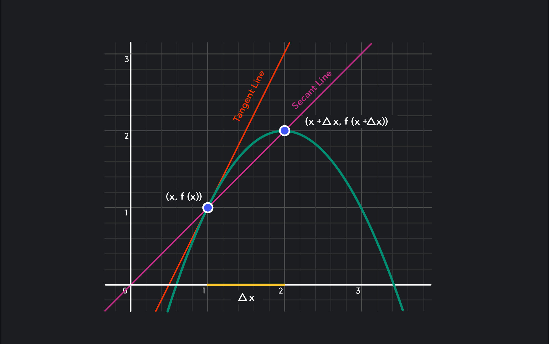
A secant line is a straight line that passes through two points on a curve. For example, the below graph of a function illustrates the secant line through $x = 1$ and $x = 2$.

The slope of the secant line is equal to the quotient of the change in $y$ and the change in $x$.

$\text{Slope of the Secant Line} = \frac{\Delta{y}}{\Delta{x}} = \frac{y_2 - y_1}{x_2-x_1} = \frac{{f\left( {x + \Delta{x} } \right) - f\left( x\right)}}{\Delta{x} }$

Both the numerator and denominator should look very familiar—the equation for the slope of the secant line is equal to the average rate of change over $[x, x + \Delta{x}]$!

So, the slope of the secant line gives us the slope between two points on a curve. But what if we want to find the slope of the curve at a single point, instead of between two points?

To find the slope of a curve at a single point, we must find the slope of the tangent line at that point. A tangent line touches the curve at just one point and also matches the direction of the curve at that point.

Consider again the secant line on the graph, as well as $\Delta{x}$ on the x-axis. Imagine making $\Delta{x}$ smaller and smaller until it nearly reaches zero. Visualize how the secant line would change at each alteration so that it matches the direction of the curve at $x = 1$ more and more closely each time.

As $\Delta{x}$ approaches zero, our approximation of the slope of the tangent line becomes more and more accurate. So, to find the precise slope of the curve at $x = a$, we can take the limit of the slope of the secant line through $(a, f(a))$ and $(a + \Delta{x}, f(a +\Delta{x}))$ as $\Delta{x}$ approaches zero.

Thus, the slope of the tangent line at the point $(a, f(a))$ is given by:

Notice that this formula is equal to the definition of $f’(a)$ given earlier, as well as the definition of the instantaneous rate of change given in the previous section!

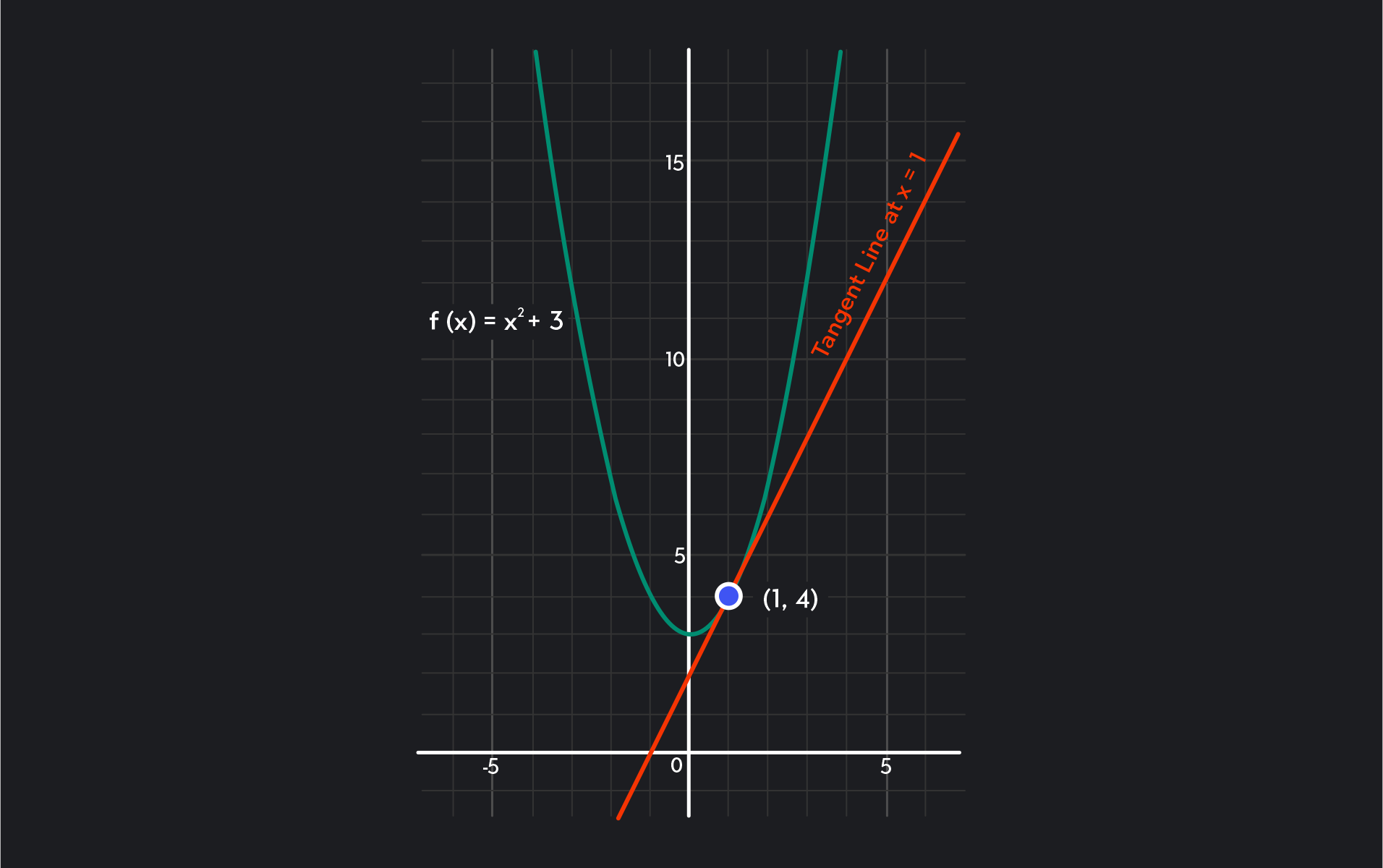
Let’s try an example. We’ll find the slope of the tangent line of the parabola $f(x) = x^2 + 3$ at $x = 1$. The graph of the function is below.

Using the definition of the slope of the tangent line, we have:

So, the slope of the tangent line is 2 at the given point $x = 1$. After determining the slope of the line, we can find the rest of the equation for the tangent line using the point-slope formula $y - y_1 = m(x - x_1)$.

Derivatives and Velocity

We can think about velocity as an extension of the “rates of change” interpretation of the derivative. Earlier, we noted that rates of change describe how much one variable changes in response to a change in another variable.

Velocity is one kind of rate of change. Velocity is the rate of change of distance over elapsed time and measures the rate at which an object changes its position regarding time.

Velocity is a vector, meaning that it has both a magnitude and a direction. The magnitude of a velocity vector is speed. The direction of a velocity vector indicates the direction in which an object is being displaced.

For example, define the polynomial $s(t) = t^2 - t - 2$ as the distance in feet of an object from its starting position, where $t$ is in seconds. We’ll find the instantaneous velocity of the object at $t = 2$ seconds.

Using the definition of instantaneous rate of change, we have:

Thus the velocity of the given function at $t = 2$ is 3 feet per second.

We’ve been using LaGrange’s notation for the derivative, which is $f’(x)$. We often read aloud this as “f prime of x.” Another common notation is Leibniz’s notation, which is $\frac{dy}{dx}$.“ We read this notation aloud as “dy dx.”

For velocity and other physics applications, we sometimes use Newton’s notation instead. Newton’s notation, or dot notation, looks like $\dot{x}$, and places a dot over the dependent variable.

Acceleration is the rate of change of velocity. We can think about acceleration as the second derivative of a function. In particular, acceleration is the second derivative of position with respect to time. Second derivatives are an example of higher-level derivatives and can be found by taking the derivative of the first derivative. Higher-level derivatives give us interesting information about the behavior of a function, such as concavity.

Explore Outlier's Award-Winning For-Credit Courses

Outlier (from the co-founder of MasterClass) has brought together some of the world's best instructors, game designers, and filmmakers to create the future of online college.

Check out these related courses:

Calculus I

The mathematics of change.

Explore course

Calculus I

The mathematics of change.

Explore course

Intro to Statistics

How data describes our world.

Explore course

Intro to Statistics

How data describes our world.

Explore course

Intro to Microeconomics

Why small choices have big impact.

Explore course

Intro to Microeconomics

Why small choices have big impact.

Explore course