How to Find Limits in Calculus

In This Article

1. What Is a Limit?

2. How to Find Limits

3. Practice Exercises and Solutions

What Is a Limit?

Before getting into how to find a limit, let’s first define a limit. Given a function $f$, a limit is the word used to describe the value that $f(x)$ tends towards as $x$ tends towards some value. The notation for the limit of a function $f$ as $x$ approaches some number $c$ looks like this:

You can read the above notation as, “The limit of $f(x)$ as $x$ approaches $c$ equals $L$.”

In other words, $f(x)$ tends towards $L$ as $x$ tends towards $c$.

How to Find Limits

When finding limits, there are several methods we can use. We will go over six possible methods:

• Direct Substitution

• Factorization

• Rationalization

• The Squeeze Theorem

• Trigonometric Identities

• L'Hôpital's Rule

• The method we use to find the limit, however, will depend on the type of function.

Direct Substitution

The term direct substitution is exactly as it sounds; you directly substitute a given value into a limit. Now, when do we need this method? If your function $f$ is continuous, the value of $f$ at $c$ and the limit of $f(x)$ as $x$ approaches $c$ are the same. In other words, $\lim_{x\to c}f(x) = f(c)$.

This rule is always true for polynomials, since polynomials are always continuous. Then, to evaluate a continuous function, we can simply substitute into $f(x)$ the value at which we want to find the limit.

Example 1

For example, evaluate $\lim_{x\to 0 } (x^2 + x + 10)$. Since $f(x)$ is a polynomial, we know that $f(x)$ is continuous. So, we can simply substitute $x = 0$ into $f(x)$!

It’s worth noting that the value of $f$ at $c$ and the limit of $f(x)$ as $x$ approaches $c$ are not always the same. We can often evaluate the limit of $f(x)$ as $x$ approaches $c$ even if $f(c)$ is undefined.

Example 2

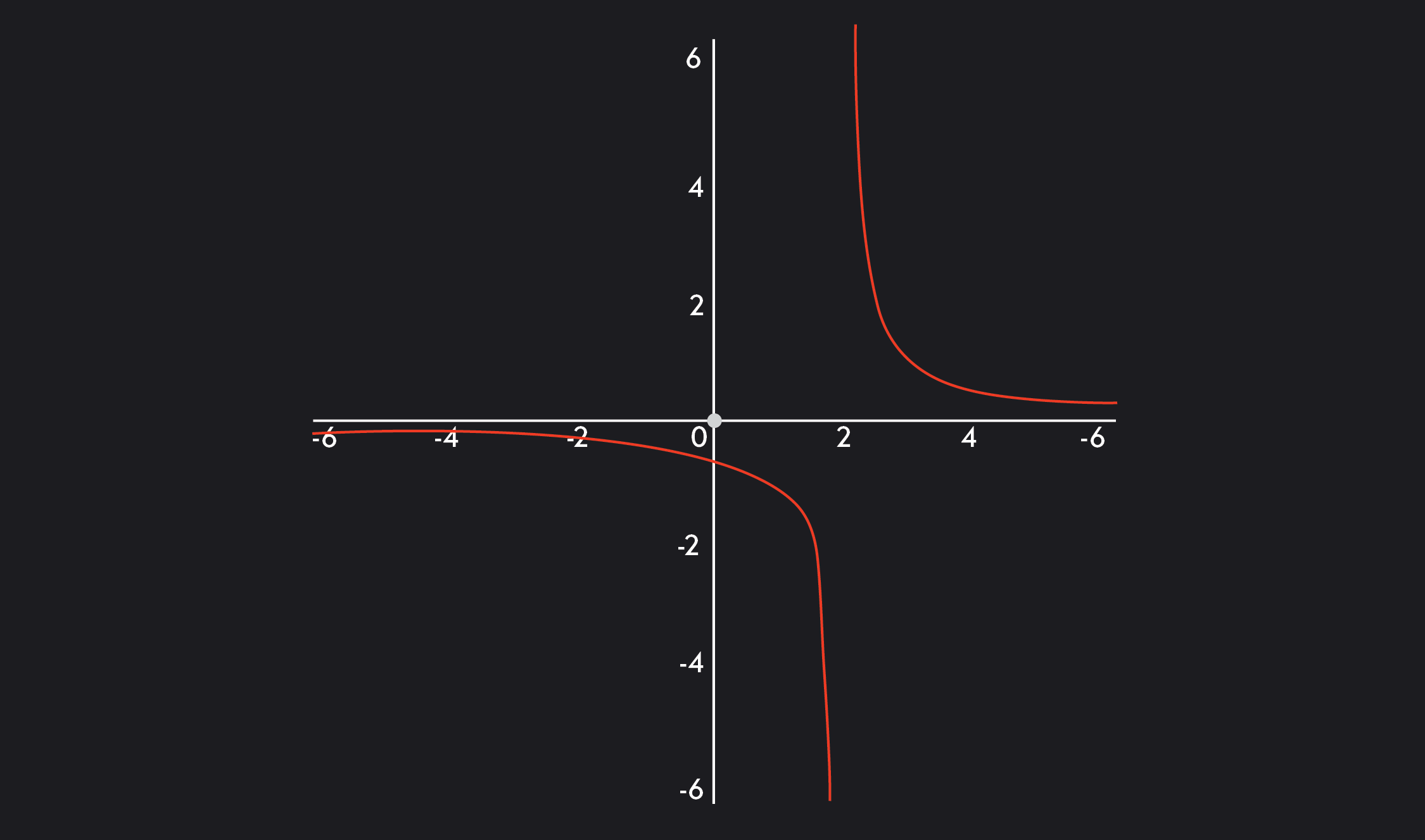
For another example, consider the rational function $f(x) = \frac{1}{x-2}$. We can’t have a denominator of zero, so $f(2)=\frac{1}{2-2}=\frac{1}{0}$ is undefined.

However, we can still evaluate the one-sided limits of $f(x)$ as $x$ approaches 2, even though $f(2)$ is undefined.

The term "one-sided limits" refers to:

• The left-sided limit, $\lim_{x\to c^- }f(x)$. This is the limit as $x$ approaches some value $c$ from the left.

• The right-sided limit, $\lim_{x\to c^+ }f(x)$. This is the limit as $x$ approaches some value $c$ from the right.

Take a look at the graph of $f(x) = \frac{1}{x-2}$ below.

Look closely at the behavior of the function near $x = 2$. The variable $x$ moves infinitely closer to 2 from both sides, yet never reaches 2.

As $x$ approaches 2 from the left, $y$ gets infinitely smaller.

As $x$ approaches 2 from the right, $y$ gets infinitely bigger. Then, the following one-sided limits are true:

Since the one-sided limits approach $+ \infty$ and $- \infty$, we say there is a vertical asymptote at $x=2$. For this example, the limit of $f(x)$ as $x$ approaches 2 does not exist, since $\lim_{x\to 2^+ }f(x) \neq \lim_{x\to 2^- }f(x)$.

For other examples, the limit will exist where there is a vertical asymptote, provided that $\lim_{x\to a^+ }f(x) = \lim_{x\to a^-}f(x)$. In order for a limit to exist, the one-sided limits must always equal each other. If the limit exists at a vertical asymptote, the value of that limit will always be $+ \infty$ or $- \infty$. Usually, if you substitute $x=a$ into $f(x)$ and get that the denominator is zero while the numerator is non-zero, that’s a good sign that there’s a vertical asymptote at $x = a$.

To give a more precise definition, we have this rule:

If any of the following statements are true, then $x=a$is a vertical asymptote of $f(x)$.

• $\lim_{​x\rightarrow a}f(x)=\infty$

• $\lim_{​x\rightarrow a}f(x)=-\infty$

• $\lim_{​x\rightarrow a^+}f(x)=\infty$

• $\lim_{​x\rightarrow a^+}f(x)=-\infty$

• $\lim_{​x\rightarrow a^-}f(x)=\infty$

• $\lim_{​x\rightarrow a^-}f(x)=-\infty$

Example 3

Let’s try direct substitution with one more example.

Let $f(x) = \frac{x^2+x-6}{x-2}$.

Evaluate $\lim_{x\to 2 }f(x)$.

Trying direct substitution, we find that $f(2) = \frac{2^2+2-6}{2-2} = \frac{6-6}{0} = \frac{0}{0}$.

When evaluating limits, we say that $\frac{0}{0}$ is indeterminate. This means that $\frac{0}{0}$ does not give us a precise enough idea of how $f(x)$ behaves as $x$ approaches 2.

Since we define division as simply the inverse of multiplication, we can say that $n = \frac{0}{0}$ implies that $0 = n \cdot 0$ for any real number $n$.

Since any number multiplied by 0 is simply 0, there are an infinite number of answers. So, $\frac{0}{0}$ is indeterminate and indicates that we’ll need to use a different method listed below.

Factorization

When direct substitution gives us an indeterminate form like $\frac{0}{0}$, we can try factoring. Factoring allows us to cancel factors that are common to both the numerator and the denominator and then apply the Quotient Rule.

The Quotient Rule states that $\lim_{x\to a}\frac{f(x)}{g(x)} = \frac{ \lim_{x\to a}f(x)}{ \lim_{x\to a}g(x)}$, given that $\lim_{x\to a}g(x) \neq 0$. Said more simply, the limit of a quotient is the quotient of the limits, provided that the denominator is non-zero.

The Quotient Rule often allows us to apply direct substitution after factoring.

Let’s try factoring our last example, where we wanted to evaluate $\lim_{x\to 2 }\frac{x^2+x-6}{x-2}$.

$\lim_{x\to 2 }\frac{x^2+x-6}{x-2} = \lim_{x\to 2 }\frac{(x+3)(x-2)}{(x-2)} = \lim_{x\to 2 }\frac{(x+3)}{1} = (2+3) = 5$

Thus, $\lim_{x\to 2 }\frac{x^2+x-6}{x-2} = 5$.

Rationalization

When dealing with limits that have radicals, it’s useful to move the radical from the numerator to the denominator or vice versa. To do this, we use rationalization. This technique involves multiplying by the conjugate. We can find the conjugate of an expression by switching the sign in the middle of the expression.

For example, let’s evaluate $\lim_{x\to 0}\frac{\sqrt{x+1}-1}{x}$. Since substituting in $x = 0$ gives us $\frac{0}{0}$, we’ll try multiplying by the conjugate of the numerator.

Thus, $\lim_{x\to 0}\frac{\sqrt{x+1}-1}{x} = \frac{1}{2}$.

The Squeeze Theorem

The Squeeze Theorem is a method where we “sandwich” a function between two easier ones in order to evaluate its limit. This method states that if we can find two functions $f(x)$ and $h(x)$ that “squeeze” or trap $g(x)$ between them on some interval $[a, b]$, and if $f(x)$ and $h(x)$ have the same limit $L$ at $c$, then $g(x)$ must also have the same limit $L$ at $c$.

More precisely, if $f(x) \leq h(x) \leq g(x)$ for all $x$ on $[a, b]$ (except possibly at $x = c$), and $\lim_{x\to c}f(x) = \lim_{x\to c}g(x) = L$, then $\lim_{x\to c}h(x) = L$

Again, the Squeeze Theorem traps one tricky function between two easier functions.

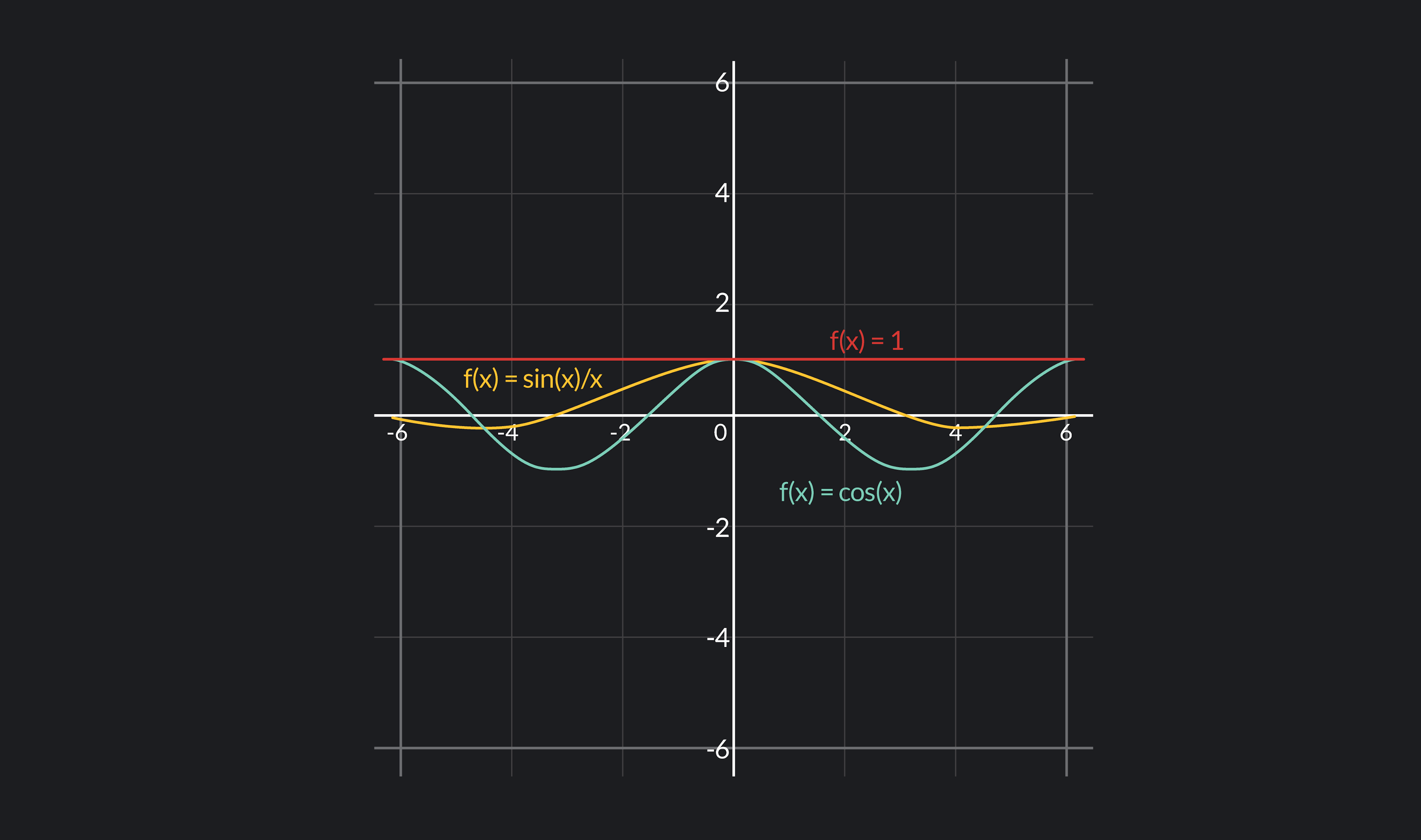
Using the Squeeze Theorem, let’s evaluate $h(x) = \lim_{x\to 0}\frac{\sin (x)}{x}$.

We need to trap $h(x)$ between two easier functions. To find these functions, look at the graph below, which graphs $f(x) = \cos (x)$, $g(x) = 1$, and $h(x) = \frac{\sin (x)}{x}$.

Using this graph, we can say that $\cos (x) \leq \frac{\sin (x)}{x} \leq 1$.

Now, note that:

Since $h(x) = \frac{\sin (x)}{x}$ is sandwiched between $f(x) = \cos (x)$ and $g(x) = 1$, and since $\lim_{x\to 0}f(x) = \lim_{x\to 0}g(x) = 1$, the Squeeze Theorem says that $\lim_{x\to 0}\frac{\sin (x)}{x} = 1$.

Trigonometric Identities

Using trigonometric identities is another clever way to manipulate functions so that we can more easily evaluate the limit. Trigonometric identities are rules involving trigonometric functions that are always true. These equations can be substituted into trigonometric functions to make the problem easier.

While there are many different trigonometric identities, familiarizing yourself with them all is a worthwhile endeavor.

Some identities are for evaluating trigonometric functions are:

• Pythagorean Identities

• Reciprocal Identities

• Double Angle Identities

• Quotient Identities

For this example, we’ll look at a Pythagorean identity.

Let $f(x) = \frac{1-\cos{(x)}}{x}$. Let’s evaluate $\lim_{x\to 0 }f(x)$.

Plugging in $x=0$ gives us $f(x) = \frac{0}{0}$, so we’ll have to find another way.

First, let’s multiply by the conjugate of the numerator. We can find the conjugate of the numerator by simply switching the sign in the middle of the expression. Multiplying by the conjugate is a very handy tool that allows us to discover trigonometric identities that aren’t obvious in the original form of the given function. In this problem, we’ll use a Pythagorean identity, which states that $\sin ^2 (x) + \cos ^2 (x) = 1$. So, we have:

By the Product Rule, we know that:

$\lim_{x\to 0}\frac{\sin (x)}{x} \cdot \frac{\sin (x)}{1 + \cos (x)} = \lim_{x\to 0}\frac{\sin (x)}{x} \cdot \lim_{x\to 0}\frac{\sin (x)}{1 + \cos (x)}$

And, using our answer from the Squeeze Theorem example, we know that $\lim_{x\to 0}\frac{\sin (x)}{x} = 1$. Then, we have:

Thus, $\lim_{x\to 0}\frac{1-\cos{(x)}}{x} = 0$.

L'Hôpital's Rule

L'Hôpital's Rule states that $\lim_{x\to\infty}\frac{f(x)}{g(x)} = \lim_{x\to\infty}\frac{f’(x)}{g’(x)}$ if the first limit $\lim_{x\to a}\frac{f(x)}{g(x)}$ is indeterminate. This means that when direct substitution gives us an indeterminate form, we can differentiate the numerator and denominator, and then take the same limit again. 

For example, evaluate $\lim_{x\to 2}\frac{x-2}{x^2-4}$. Direct substitution gives us $\frac{0}{0}$, so we’ll try L'Hôpital's Rule. Let $f(x)$ be the numerator and $g(x)$ be the denominator.

Thus, $\lim_{x\to 2}\frac{x-2}{x^2-4}=\frac{1}{4}$.

Practice Exercises and Solutions

Now that we’ve seen how to evaluate limits, here are exercises where you can practice how to find the limit of a function.

Exercise 1

Evaluate $\lim_{x\to 1}\frac{1}{(x-1)^2}$.

What does this limit suggest?

Solution:

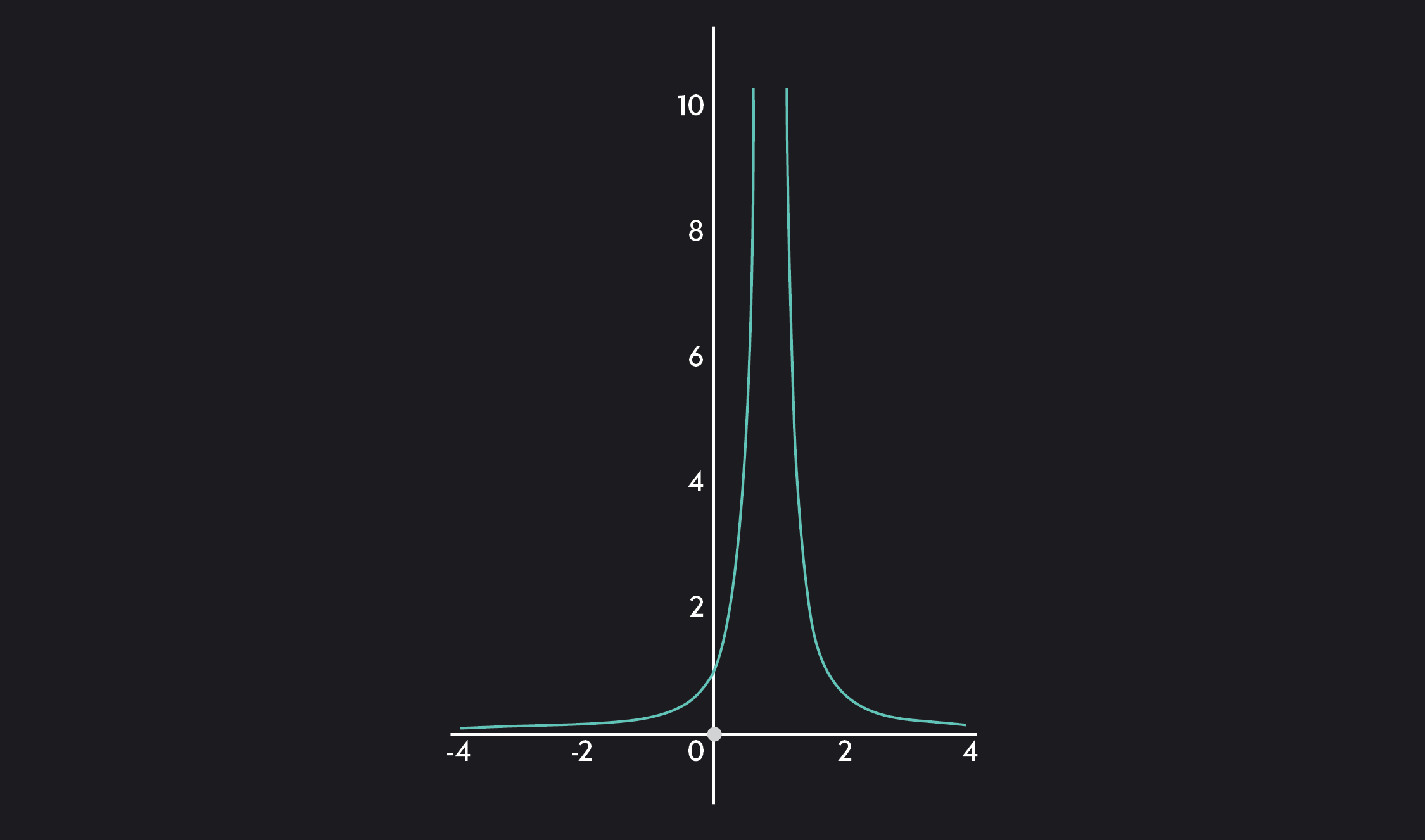
When we plug $x = 1$ into $f(x) = \frac{1}{(x-1)^2}$, we find that $f(1) = \frac{1}{0}$. This is a good indication that there may be a vertical asymptote at $x = 1$.

Looking at the graph of $f(x)$, we see that $y$ approaches $+\infty$ as $x$ approaches 1 from the left.

And, $y$ approaches $+\infty$ as $x$ approaches 1 from the right. Thus, $\lim_{x\to 1}\frac{1}{(x-1)^2} = \infty$, and there is a vertical asymptote at $x = 1$.

Exercise 2

Evaluate $\lim_{x\to -1}\frac{x^2-5x-6}{x+1}$.

Solution:

Direct substitution gives us $\lim_{x\to -1}\frac{x^2-5x-6}{x+1} = \frac{0}{0}$, so we’ll try factoring. Then, we have:

Exercise 3

Evaluate $\lim_{x\to 4}\frac{\sqrt{x}-2}{x-4}$.

Solution:

Direct substitution gives us $\frac{0}{0}$, so we’ll use rationalization to solve this problem. To rationalize the radical in the numerator, we’ll multiply by its conjugate.

Exercise 4

Evaluate $\lim_{x\to 0} x^2 \cos (\frac{1}{x})$.

Solution:

For this problem, we’ll use the Squeeze Theorem. We need to trap $h(x) = x^2 \cos (\frac{1}{x})$ between two easier functions.

$\lim_{x\to 0}(-x^2) = 0$ and $\lim_{x\to 0}(x^2) = 0$

Since $h(x)$ is sandwiched between $f(x) = -x^2$ and $g(x) = x^2$ and since $\lim_{x\to 0}f(x) =\lim_{x\to 0}g(x) = 0$, then $\lim_{x\to 0} x^2 \cos (\frac{1}{x}) = 0$.

Exercise 5

Evaluate $\lim_{x\to 0} \frac{\sin (x)}{\sin (2x)}$.

Solution:

Direct substitution gives us $\frac{0}{0}$, so we’ll use trig identities to solve this problem. Specifically, it will be helpful to use a Double Angle identity, which states that $\sin (2x) = 2 \sin (x) \cos (x)$.

Exercise 6

Evaluate $\lim_{x\to 3} \frac{x^3-27}{x-3}$.

Solution:

Direct substitution gives us $\frac{0}{0}$, so we’ll use L'Hôpital's Rule. Let $f(x)$ be the numerator and $g(x)$ be the denominator.

Explore Outlier's Award-Winning For-Credit Courses

Outlier (from the co-founder of MasterClass) has brought together some of the world's best instructors, game designers, and filmmakers to create the future of online college.

Check out these related courses:

Calculus I

The mathematics of change.

Explore course

Calculus I

The mathematics of change.

Explore course

Intro to Statistics

How data describes our world.

Explore course

Intro to Statistics

How data describes our world.

Explore course

Intro to Microeconomics

Why small choices have big impact.

Explore course

Intro to Microeconomics

Why small choices have big impact.

Explore course