Continuous Functions: Definition, Examples, and Properties

In This Article

1. What is a Continuous Function?

2. What is a Discontinuous Function?

3. Properties of Continuous Functions

4. Theorems for Continuous Functions

What is a Continuous Function?

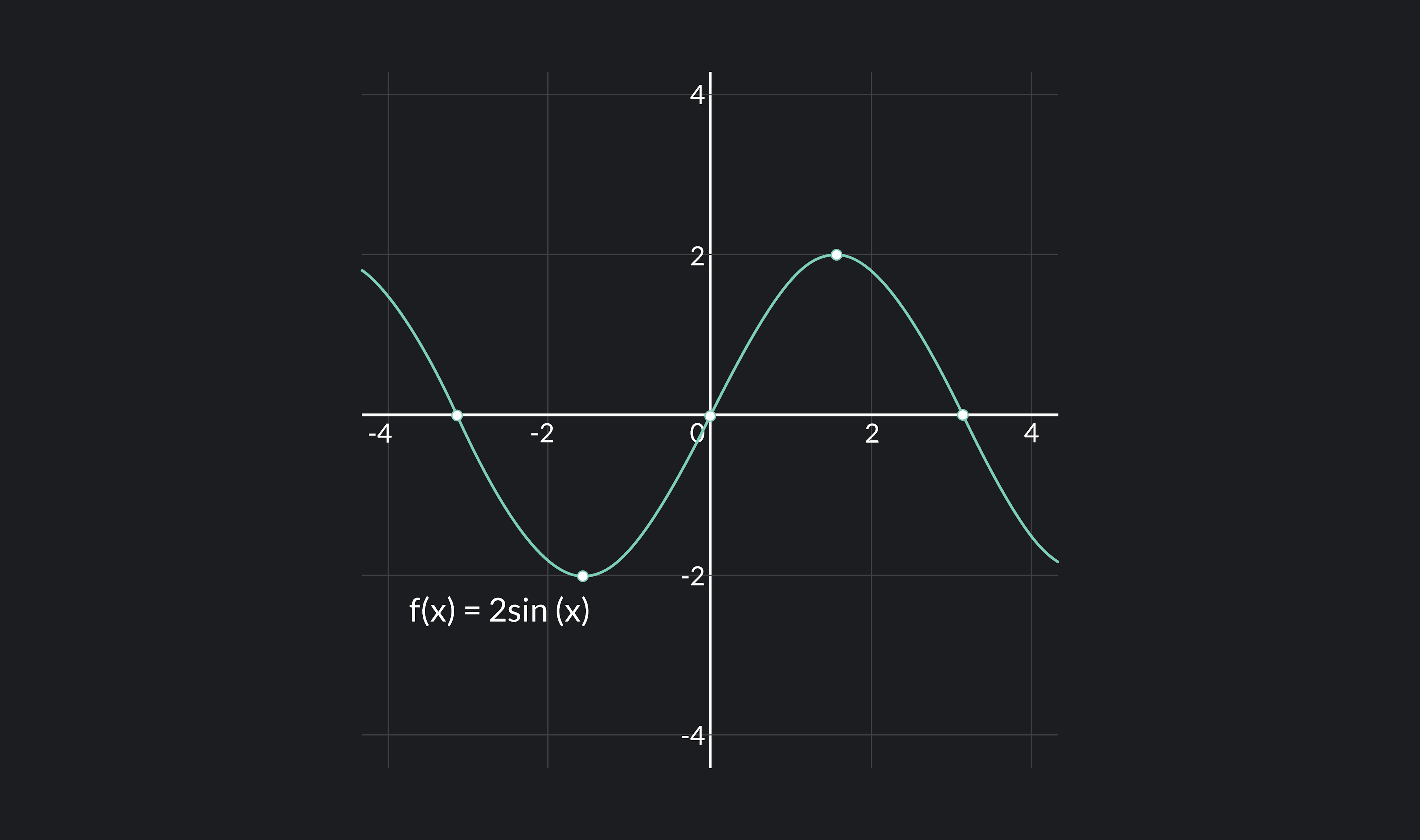
A function is continuous everywhere if you can trace its curve on a graph without lifting your pencil. A function is discontinuous at a point if you cannot trace its curve without lifting your pencil at that point; meaning it has a hole, break, jump, or vertical asymptote at that point.

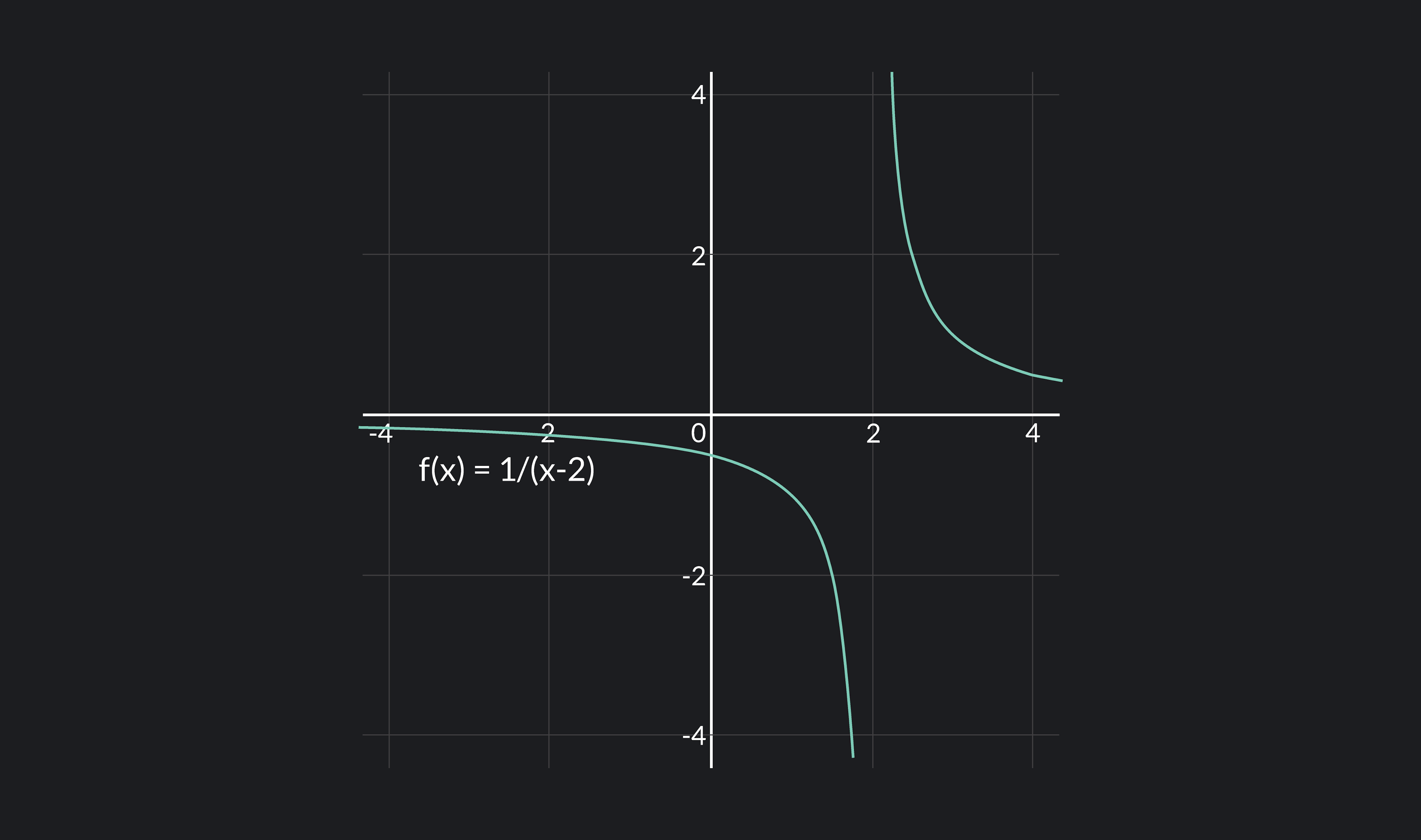
For example, the function $f(x) = 2\sin{(x)}$ is continuous everywhere. We can draw its curve without ever lifting our hand. By contrast, the function $f(x) = \frac{1}{x-2}$ has a discontinuity at $x = 2$. We can’t draw its curve without lifting our pencil at $x = 2$.

In differential calculus, it’s important to understand the concept of continuity because functions that are not continuous are not differentiable.

Let’s learn how to prove a function is continuous at a point. Here’s the formal definition of continuity at a point.

A function $f$ is continuous at the point $x = a$ if:

• $f(a)$ exists

• $\lim_{x\to a}f(x)$ exists

• $f(a) = \lim_{x\to a}f(x)$

In order to show that a function is continuous at a point $a$, you must show that all three of the above conditions are true. To refresh your knowledge of evaluating limits, you can review How to Find Limits in Calculus and What Are Limits in Calculus.

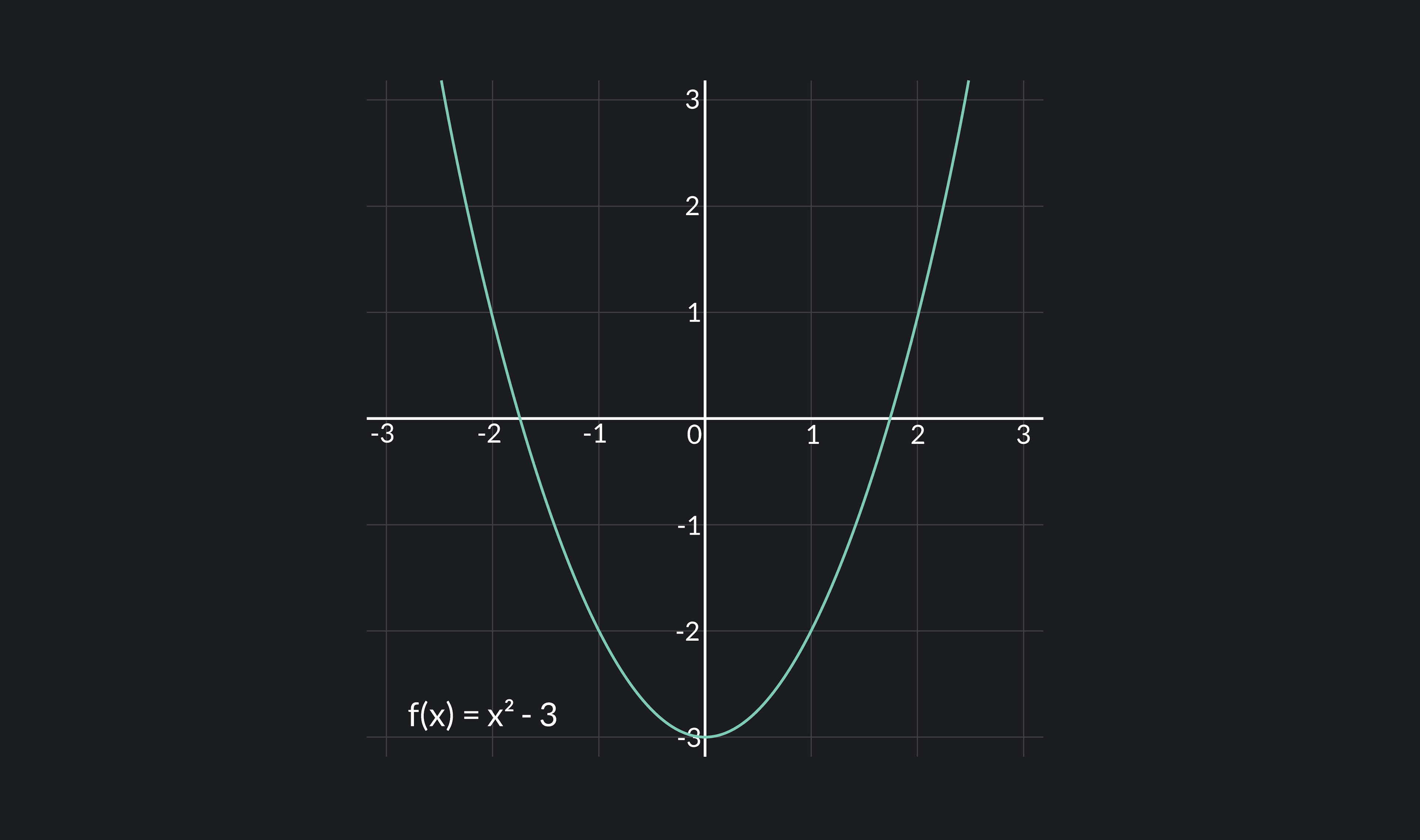
For example, let’s show that $f(x) = x^2 - 3$ is continuous at $x = 1$.

• $f(1) = 1^2 - 3 = -2$

• $\lim_{x\to 1}f(x) = -2$

• $f(1) = \lim_{x\to 1}f(x) = -2$

Thus, $f(x) = x^2 - 3$ is continuous at $x = 1$. In fact, we could show that $f(x) = x^2 - 3$ is continuous everywhere.

Other functions might be continuous only over a specific interval of the real numbers. If a function is continuous on an open interval, that means that the function is continuous at every point inside the interval.

For example, $f(x) = \tan{(x)}$ has a discontinuity over the real numbers at $x = \frac{\pi}{2}$, since we must lift our pencil in order to trace its curve. However, we can say that $f(x) = \tan{(x)}$ is continuous on the open interval $(-\frac{\pi}{2}, \frac{\pi}{2})$ since it is continuous at every point inside that specific interval.

We can also say that $f(x) = \tan{(x)}$ is continuous over its own domain, which is any real number excluding odd multiples of $\frac{\pi}{2}$.

What is a Discontinuous Function?

A discontinuity is a hole, jump, break, or vertical asymptote on a function's curve.

There are 3 types of discontinuities.

Jump Discontinuities

If a function has a jump discontinuity at some point $a$, then $\lim_{x\to a}f(x)$ does not exist. Remember that in order for a limit to exist, its one-sided limits must exist and they must equal the same value. In other words, the limit as $x$ approaches $a$ from the left must equal the limit as $x$ approaches $a$ from the right.

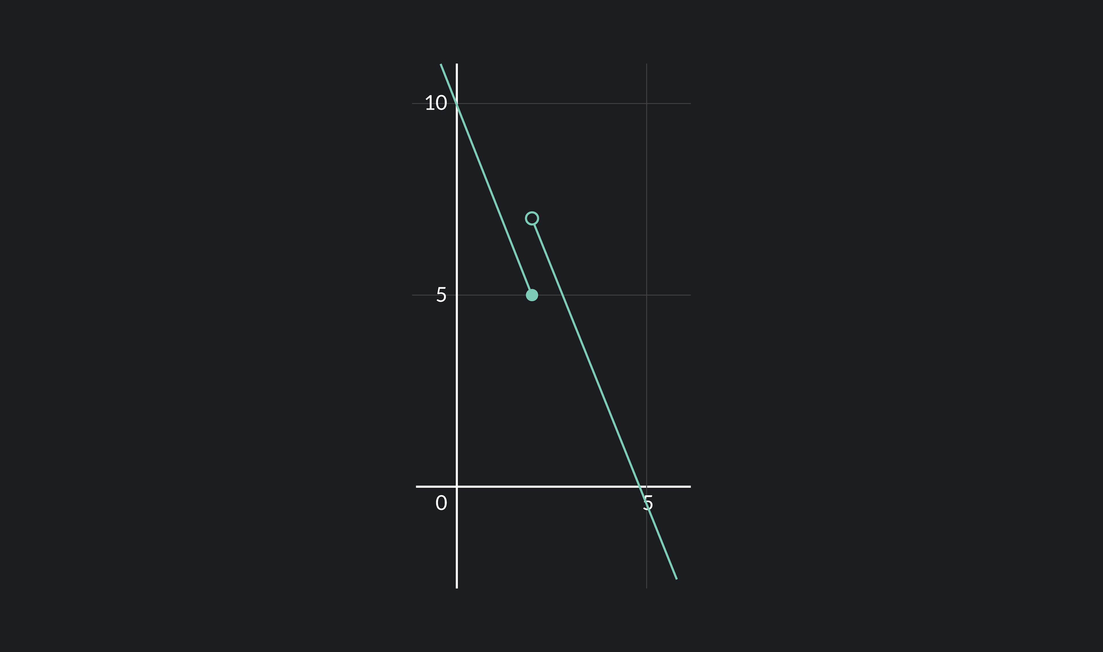
In functions with jump discontinuities, $\lim_{x\to a^+}f(x) \neq \lim_{x\to a^-}f(x)$. For example, in the function above, $\lim_{x\to 2^+}f(x) = 5$ and $\lim_{x\to 2^-}f(x) = 7$. Thus, $\lim_{x\to 2}f(x)$ does not exist, and so there is a discontinuity at $x = 2$.

Removable Discontinuities

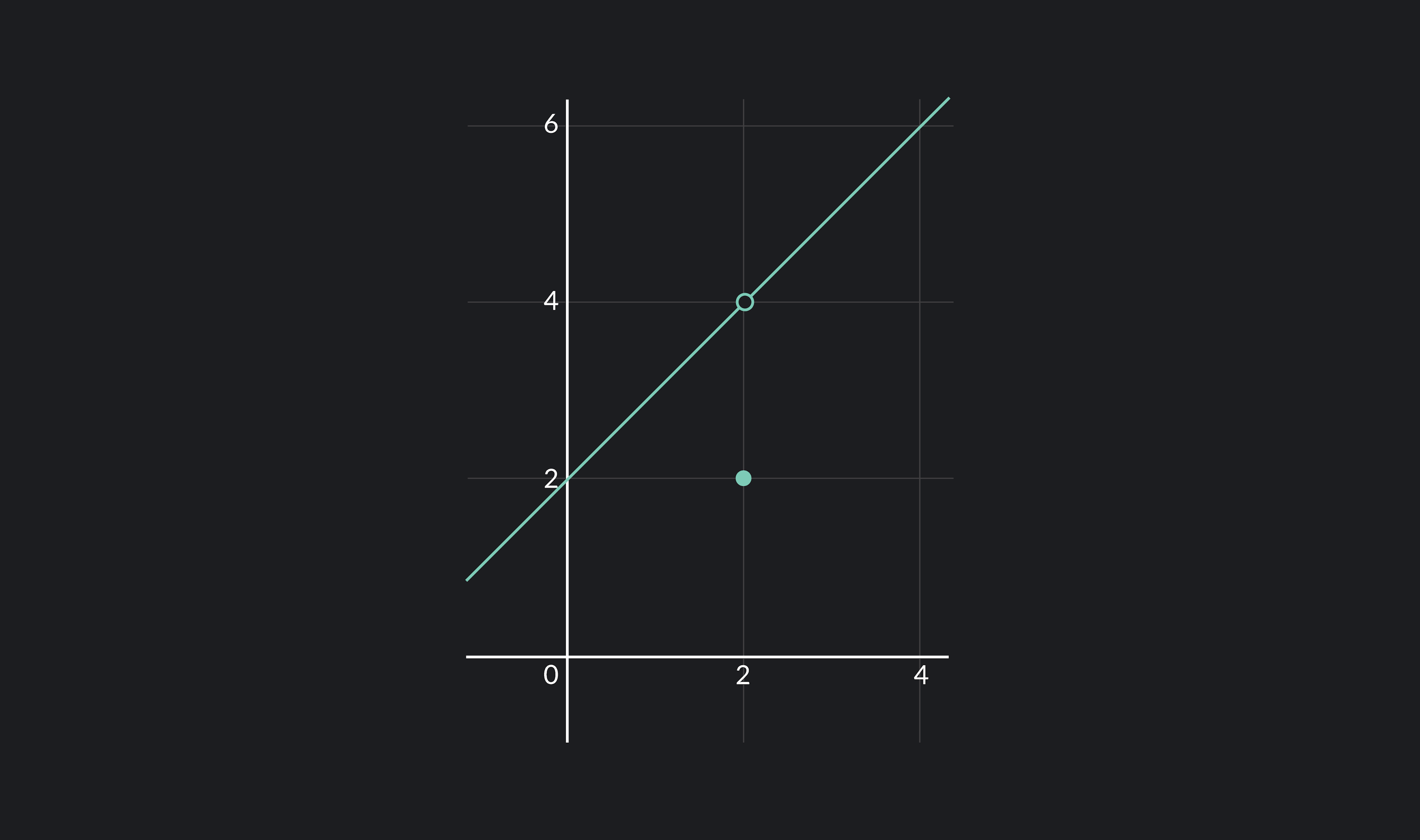
If a function has a removable discontinuity at some point $a$, then $\lim_{x\to a}f(x) \neq f(a)$. On a graph, this looks like a hole. In these discontinuities, the one-sided limits as $x$ approaches $a$ always equal each other. However, the function’s value at $x = a$ equals something different or might not exist at all.

For example, in the function above, $\lim_{x\to 2}f(x) = 4$. However, $f(2) = 2$. Since $\lim_{x\to 2}f(x) \neq f(2)$, the function has a discontinuity at $x = 2$.

Infinite Discontinuities

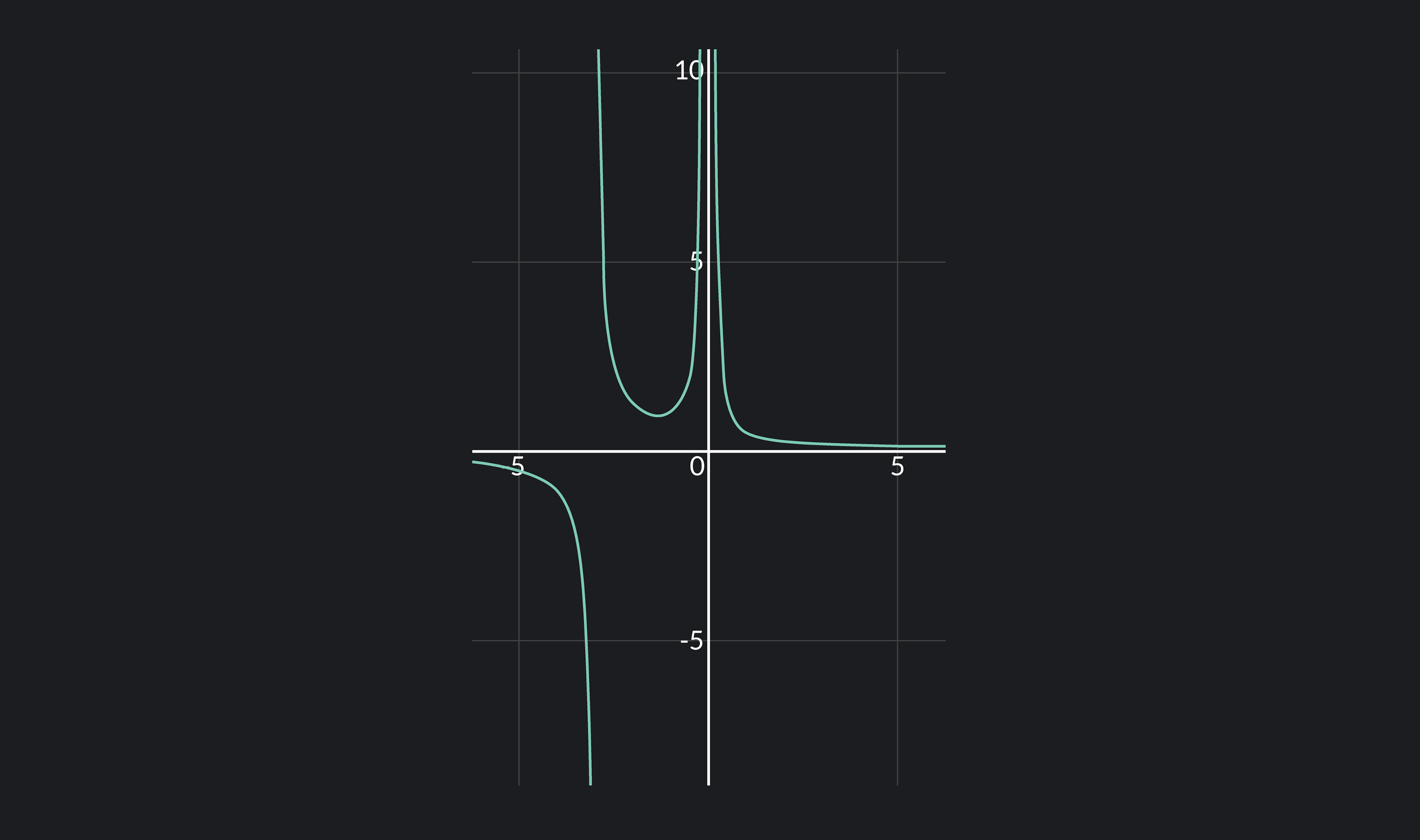
If a function has an infinite discontinuity at some point $a$, then the function has a vertical asymptote at $x = a$. If any one of the following statements are true, then $f$ has a vertical asymptote at $x = a$.

• $\lim_{x\to a^+ }f(x) = +\infty$

• $\lim_{x\to a^+ }f(x) = -\infty$

• $\lim_{x\to a^- }f(x) = +\infty$

• $\lim_{x\to a^- }f(x) = -\infty$

For example, in the function above, there is a vertical asymptote at $x = -3$ and $x = 0$. Thus, there is an infinite discontinuity at $x = -3$ and $x = 0$.

Properties of Continuous Functions

If $f$ and $g$ are both continuous at $x = c$, then the following properties are true:

• The sum $(f+g)x = f(x) + g(x)$ is continuous at $x = c$.

• The difference $(f-g)x = f(x) - g(x)$ is continuous at $x = c$.

• The product $(f \cdot g)x = f(x) \cdot g(x)$ is continuous at $x = c$.

• The quotient $(\frac{f}{g})(x) = \frac{f(x)}{g(x)}$ is continuous, provided $g(x) \neq 0$.

• The constant multiple $k \cdot f(x)$ is continuous at $x = c$ for any number $k$.

• The composition $(f \circ g)(x) = f(g(x))$ is continuous at $c$ if $f$ is continuous at $g(c)$.

Theorems for Continuous Functions

Extreme Value Theorem

The Extreme Value Theorem states that if a function is continuous on the closed interval $[a,b]$, then the function must have both a maximum and a minimum on $[a, b]$.

Intermediate Value Theorem

The Intermediate Value Theorem is an extremely useful theorem in math. It’s often used to prove that different equations are solvable. It’s especially useful for proving that a function has a root on a particular interval. The root of a function is the point at which a function equals zero and crosses the x-axis. The Intermediate Value Theorem states:

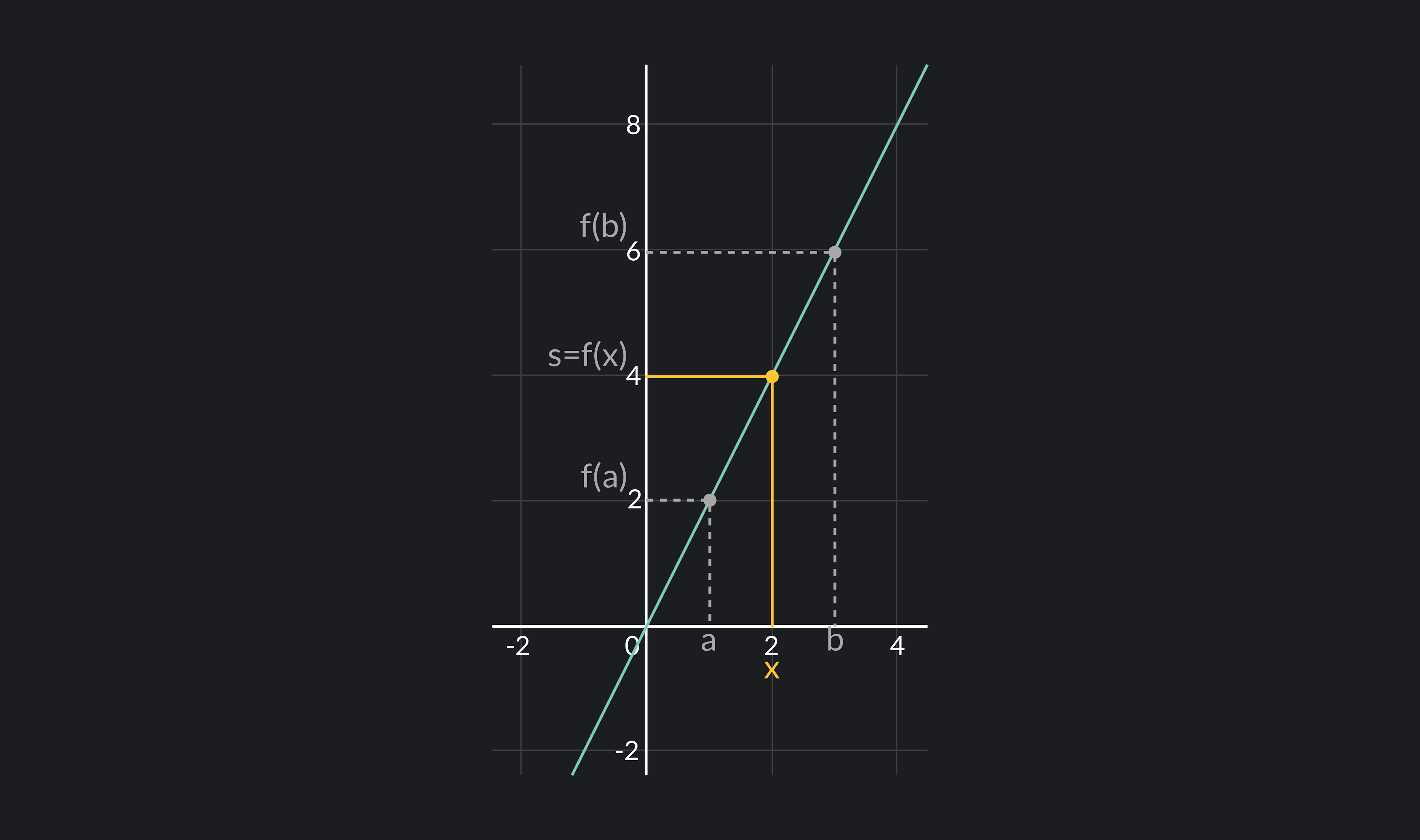
Suppose f is a continuous function defined on [a, b], and let s be a number such that f(a) < s < f(b). Then, there must exist some x between a and b such that f(x) = s.

More simply, the Intermediate Value Theorem says that a continuous function must take on every value between $f(a)$ and $f(b)$ at least once on the interval $[a, b]$.

For example, consider the graph of $f(x) = 2x$ in the above graph. Let’s examine the interval $[a, b]$ where $a = 1$ and $b = 3$. Since $f(a) = 2$ and $f(b) = 6$, we’ll choose an in-between value $s = 4$ for our s-value.

Then, since $f(x) = 2x$ is continuous on $[1, 3]$, the Intermediate Value Theorem guarantees that there must exist some $x$ on $[1, 3]$ such that $f(x) = 4$. By looking at the graph, we can see that $x = 2$ is the value for which $f(x) = s = 4$.

Polynomial Function

Any polynomial function is continuous for all real numbers. A polynomial function is a function consisting of variables and coefficients that involves only non-negative exponents of the variable. Polynomials use only addition, subtraction, and multiplication operations. For example, $f(x) = 7x^3 + x^2 - 5$ is a polynomial function.

Differentiable Function

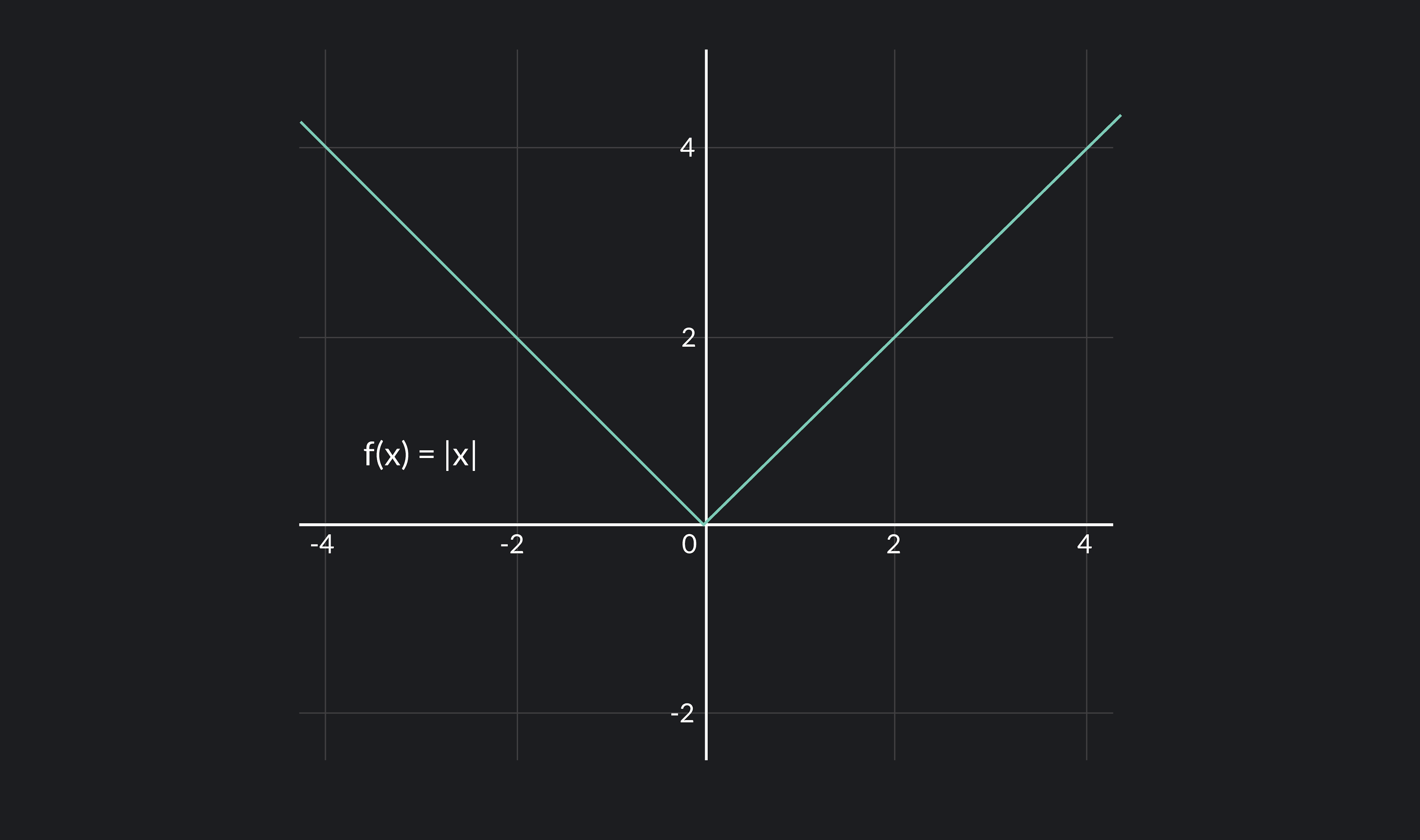
Every differentiable function is continuous. However, be careful to remember that the converse is not necessarily true. A function could be continuous, but not differentiable. For example, the absolute value function $f(x) = \mid x \mid$ below is continuous at $x = 0$ but not differentiable at $x = 0$.

Other Functions

Rational, root, trigonometric, exponential, and logarithmic functions are all continuous in their domains. The domain of a function is the set of values that a function can accept as inputs. Many real life examples of continuous functions can be modeled using these function types.

Rational Functions

A rational function is a function that is written as the ratio of two polynomial functions. The domain of rational functions is all numbers except those that make the denominator zero. So, the values where rational functions have vertical asymptotes or removable discontinuities are outside of their domain.

Trigonometric Functions

The trigonometric functions $\sin(x)$ and $\cos(x)$ have domains that include all real numbers. So, they are continuous for all real numbers.

Other trigonometric functions such as $\tan(x)$ have more selective domains — for example, the domain of $\tan(x) = \frac{\sin(x)}{\cos(x)}$ is equal to all real numbers except for where $\cos(x) = 0$. This occurs at every odd multiple of $\frac{\pi}{2}$, and so these x-values are outside the domain of $\tan(x)$.

Exponential Functions

Exponential functions have the form $f(x) = ab^x$, where $a \neq 0$ and $b$ is a real number greater than 1. The domain of exponential functions is all real numbers.

Logarithmic Functions

Logarithmic functions are only defined for positive inputs. So, the domain of logarithmic functions can be determined by solving the inequality that sets the inside terms to be greater than 0.

Explore Outlier's Award-Winning For-Credit Courses

Outlier (from the co-founder of MasterClass) has brought together some of the world's best instructors, game designers, and filmmakers to create the future of online college.

Check out these related courses:

Intro to Statistics

How data describes our world.

Explore course

Intro to Statistics

How data describes our world.

Explore course

Precalculus

Master the building blocks of Calculus.

Explore course

Precalculus

Master the building blocks of Calculus.

Explore course

Calculus I

The mathematics of change.

Explore course

Calculus I

The mathematics of change.

Explore course

Intro to Microeconomics

Why small choices have big impact.

Explore course

Intro to Microeconomics

Why small choices have big impact.

Explore course