What Is the Second Derivative Test [Full Guide]

In This Article

1. What Is the Second Derivative Test?

2. 5 Steps to Using the Second Derivative Test

3. Applications of the Second Derivative Test

4. Examples of the Second Derivative Test

What Is the Second Derivative Test?

The second derivative test is a systematic method we use to determine the nature of critical points—maximum, minimum, or neither—of a function.

This technique allows us to better understand a curve without having to construct a graph. It’s particularly useful in optimization problems, where we want to find the maximum or minimum value of a function that is subject to certain constraints.

Here is the definition of the second derivative test:

Let $f”$ exist on some open interval containing $c$ and let $f’(c) = 0$.

1. If $f”(c) > 0$, then $f(c)$ is a relative minimum.

2. If f”(c) < 0, then f(c) is a relative maximum.

3. If $f”(c) = 0$ or $f’’(c)$ does not exist, then the test is inconclusive and other methods must be used.

5 Steps to Using the Second Derivative Test

The first derivative of a function tells us when the function is increasing, decreasing, or constant. What does the second derivative tell you?

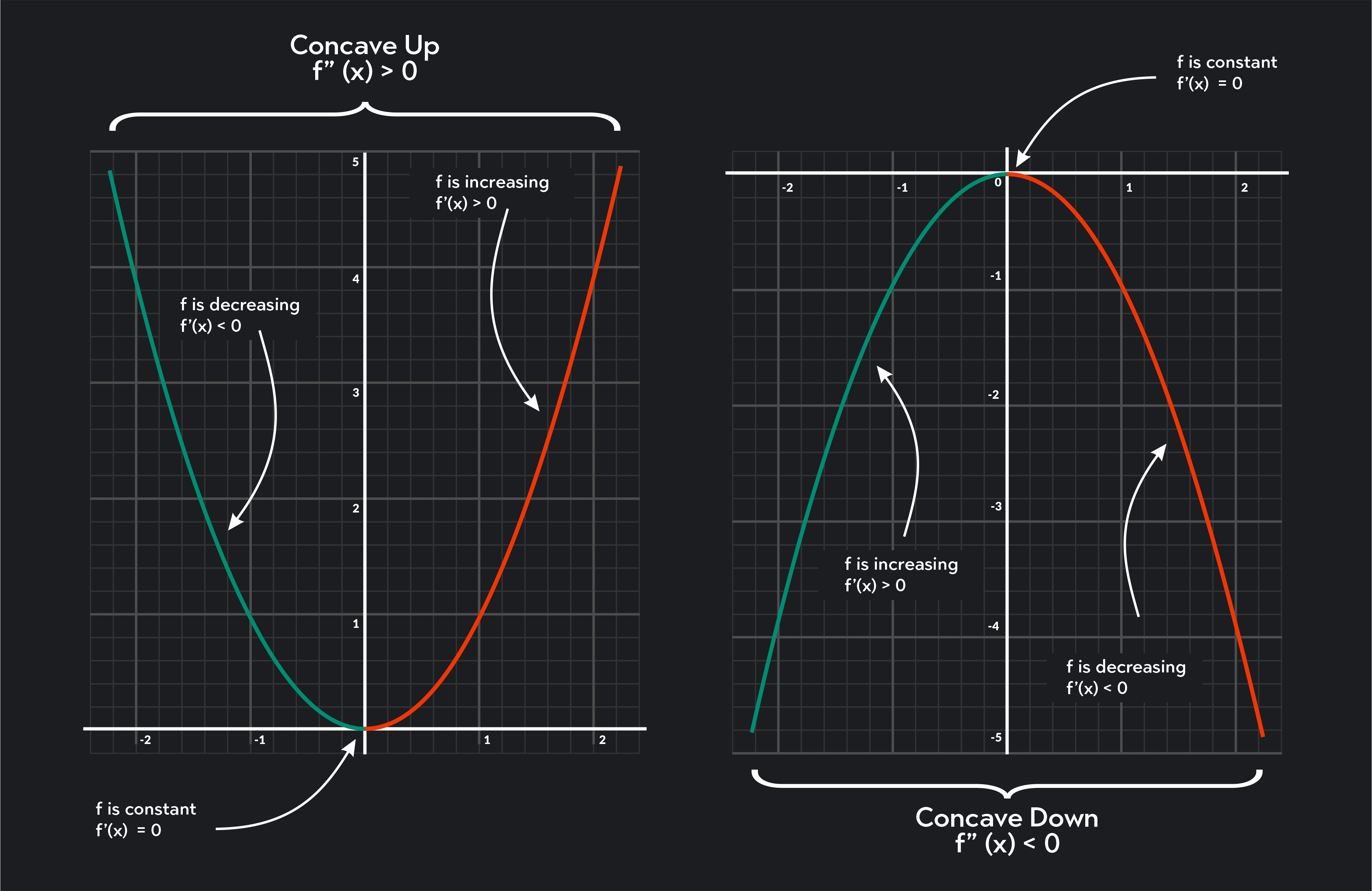
The second derivative of a function helps us to understand the shape of the curve, known as concavity. A curve’s intervals can be concave up, concave down, or have no concavity. The criteria for increasing/decreasing intervals and concave up/concave down intervals are given below:

If $f$ is a differentiable function on the interval $I$ with derivatives $f’$, then:

• If $f’(x) > 0$ for each $x$ on $I$, then $f$ is increasing on $I$.

• If f’(x) < 0 for each x on I, then f is decreasing on I.

• If $f’(x) = 0$ for each $x$ on $I$, then $f$ is constant on $I$.

If $f$ is a differentiable function on the interval $I$ with derivatives $f’$ and $f’”$, then:

• If $f”(x) > 0$ for each $x$ on $I$, then $f$ is concave up on $I$.

• If f”(x) < 0 for each x on I, then f is concave down on I.

• If $f”(x) = 0$ for each $x$ on $I$, then $f$ has no concavity.

These concepts are graphed below. Notice that there is a local minimum at $x$ when $f’(x) = 0$ and $f$ is concave up. There is a local maximum at $x$ when $f’(x) = 0$ and $f$ is concave down. This is a good way to visualize the second derivative test.

Here are the five steps to using the second derivative test. This involves learning how to find the second derivative and understanding how to identify critical points.

Step 1

Take the first derivative of the function.

Step 2

Find the critical points of the function where the first derivative is zero. The critical points where $f’(x) = 0$ are also called stationary points. To find the stationary points, set the first derivative equal to zero and solve for $x$.

Step 3

Take the second derivative of the function. To do this, take the derivative of the first derivative.

Step 4

For each stationary point $x$, plug $x$ into the second derivative function, and interpret the results.

• If $f"(x)$ is positive, then the function has a relative minimum at $x$.

• If $f"(x)$ is negative, then the function has a relative maximum at $x$.

• If $f"(x)$ is zero or non-existent at $x$, then the test is inconclusive.

When the second derivative test fails, other methods must be used to determine if there is local extrema at the critical point, such as the first derivative test.

Step 5

If desired, verify your results by graphing or using the first derivative test.

Let’s elaborate a bit more on critical points. In calculus, critical points are points on a function where the first derivative is zero or undefined. They are important because they help us to find relative extrema—local minima and local maxima.

If we think about this concept graphically, critical points are points where the slope of the tangent line to the graph of the function is either zero or undefined. At a local maximum or minimum, the tangent line is horizontal, so the slope equals zero.

To find the critical points of a function, we can take the derivative of the function and solve for the values of $x$ where the derivative is zero or undefined. These critical numbers can then be further analyzed using the second derivative test to determine whether they correspond to maxima, minima, or points of inflection.

Keep in mind that critical points and inflection points are separate concepts. The points where a function changes concavity are called inflection points. These points occur where $f”(x)$ changes sign.

On a second derivative graph, the point of inflection second derivatives have would appear as the points where the curve crosses the x-axis, or is undefined. So, if $x$ is an inflection point of $f$, then $f”(x) = 0$ or $f”(x)$ is undefined.

Examples of the Second Derivative Test

Let’s walk through a few second derivative test examples together, using the five second derivative test steps.

Example Problem 1

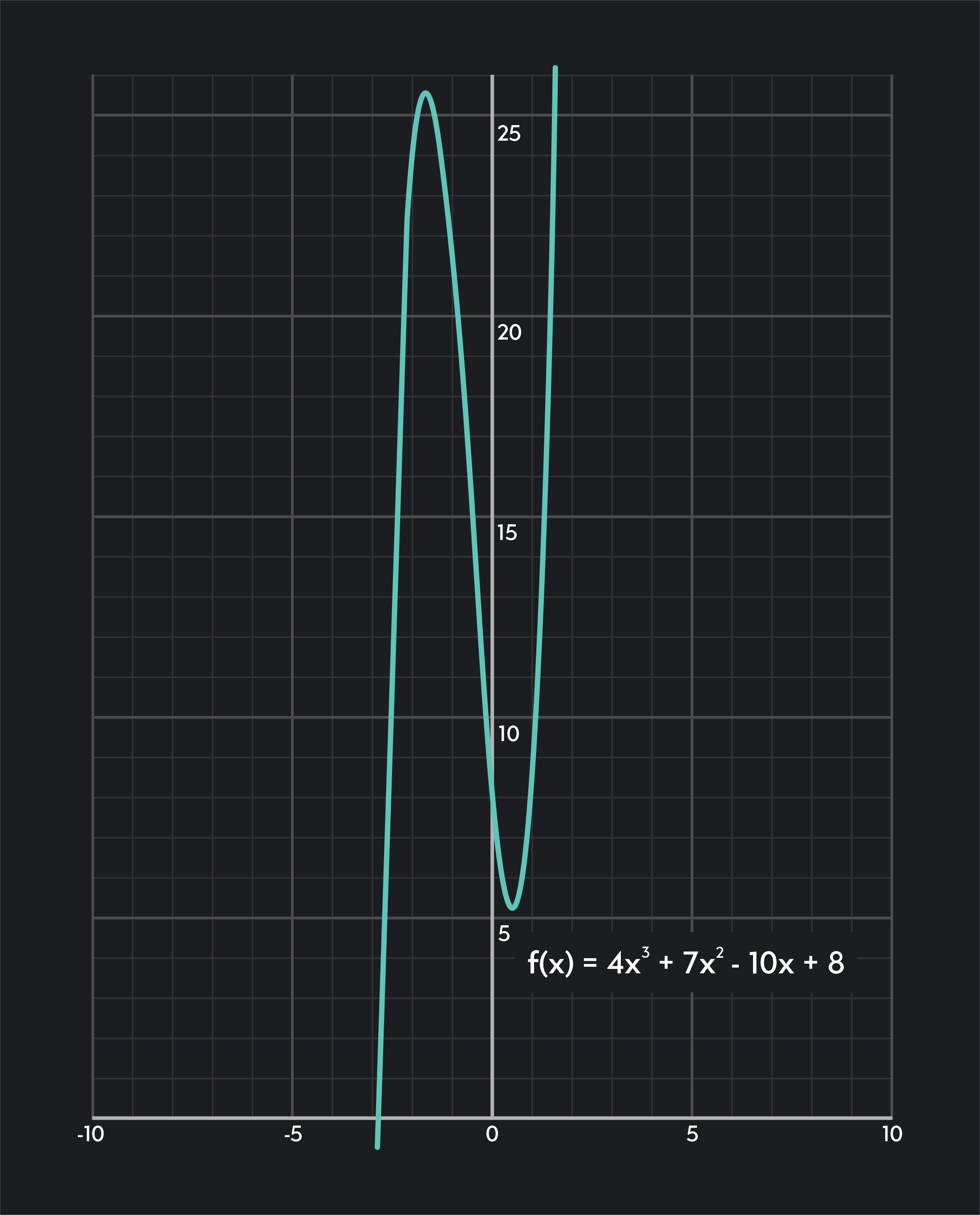
Find all relative extrema for $f(x) = 4x^3 + 7x^2 - 10x + 8$.

Step 1

Take the first derivative of the function. Using the power rule, $f’(x) = 12x^2 + 14x - 10$.

Step 2

Identify the stationary points of the function. We can do this by equating our first derivative equation to 0. Then, we’ll use factoring to solve the equation:

The two equations above give us two critical points, $x = -\frac{5}{3}$ and $x = \frac{1}{2}$.

Step 3

Take the second derivative of the function. Using the power rule, $f”(x) = 24x + 14$.

Step 4

Plug our critical points into the second derivative function, and interpret the results.

• $f”(-\frac{5}{3}) = 24(-\frac{5}{3}) + 14 = -40 + 14 = -26$

• $f”(\frac{1}{2}) = 24(\frac{1}{2}) + 14 = 12 + 14 = 26$

Since f”(-\frac{5}{3}) = -26 and -26 < 0, there is a relative maximum at -\frac{5}{3} by the second derivative test. Since f”(\frac{1}{2}) = 26 and 26 > 0, there is a relative minimum at f(\frac{1}{2}) by the second derivative test.

Step 5

Verify our results. We can do this by looking at a graph of our function. Notice that there is a local maximum at $f(-\frac{5}{3})$ and a local minimum at $f(\frac{1}{2})$.

Example Problem 2

Find all relative extrema for $f(x) = (x + 3)^4$

Step 1

Take the first derivative of the function. Using the chain rule, $f’(x) = 4(x + 3)^3$.

Step 2

Identify the stationary points of the function. We can do this by equating our first derivative equation to 0.

Step 3

Take the second derivative of the function. Using the chain rule, $f”(x) = 12(x + 3)^2$.

Step 4

Plug our critical point into the second derivative function, and interpret the results.

In this case, the second derivative test fails, since our result is 0.

To solve this problem, we need to use the first derivative test instead. To do this, we’ll examine two points on either side of $x = -3$:

These results indicate that f is decreasing on (-\infty, -3) and increasing on (-3, \infty). Thus, a relative minimum occurs at f(-3).

Applications of the Second Derivative Test

We use the second derivative test in many fields of science, including economics, physics, and engineering.

Here are 4 applications of the second derivative test:

Optimization Problems

Optimization problems involve finding the maximum or minimum value of a function that is subject to certain constraints. The second derivative test can help us determine whether a critical point is a maximum or a minimum. That way we can find the optimal solution.

Curve Sketching

When sketching the graph of a function, it's helpful to identify its critical points, and determine whether they correspond to a maximum or minimum. The second derivative test helps us to determine whether to sketch a concave up or concave down curve.

Economics

In economics, the second derivative test can be used to analyze the behavior of cost and revenue functions. For example, the second derivative test can be used to determine the level of production that will maximize profit.

Physics

The second derivative test can be used in physics to analyze the behavior of motion functions. For example, if the second derivative of a position function is positive, it indicates that the object is accelerating in the positive direction, while a negative second derivative indicates that the object is accelerating in the negative direction.

Explore Outlier's Award-Winning For-Credit Courses

Outlier (from the co-founder of MasterClass) has brought together some of the world's best instructors, game designers, and filmmakers to create the future of online college.

Check out these related courses:

Calculus I

The mathematics of change.

Explore course

Calculus I

The mathematics of change.

Explore course

Intro to Statistics

How data describes our world.

Explore course

Intro to Statistics

How data describes our world.

Explore course

Intro to Microeconomics

Why small choices have big impact.

Explore course

Intro to Microeconomics

Why small choices have big impact.

Explore course