The Arc-Length Formula: A Step-By-Step Guide

In This Article

1. The Arc Length Formula

2. How To Find the Arc Length of a Function

3. What Is the Surface Area of the Surface of Revolution?

4. How To Calculate the Surface Area of a Surface of Revolution

The Arc Length Formula

The arc length of a function is the length of the function’s curve between two points.

In order to calculate the arc length of a function $f$ on $[a, b]$, we require two things: the function must be differentiable on $[a, b]$ and its derivative must be continuous on $[a, b]$. Functions with these characteristics are called smooth.

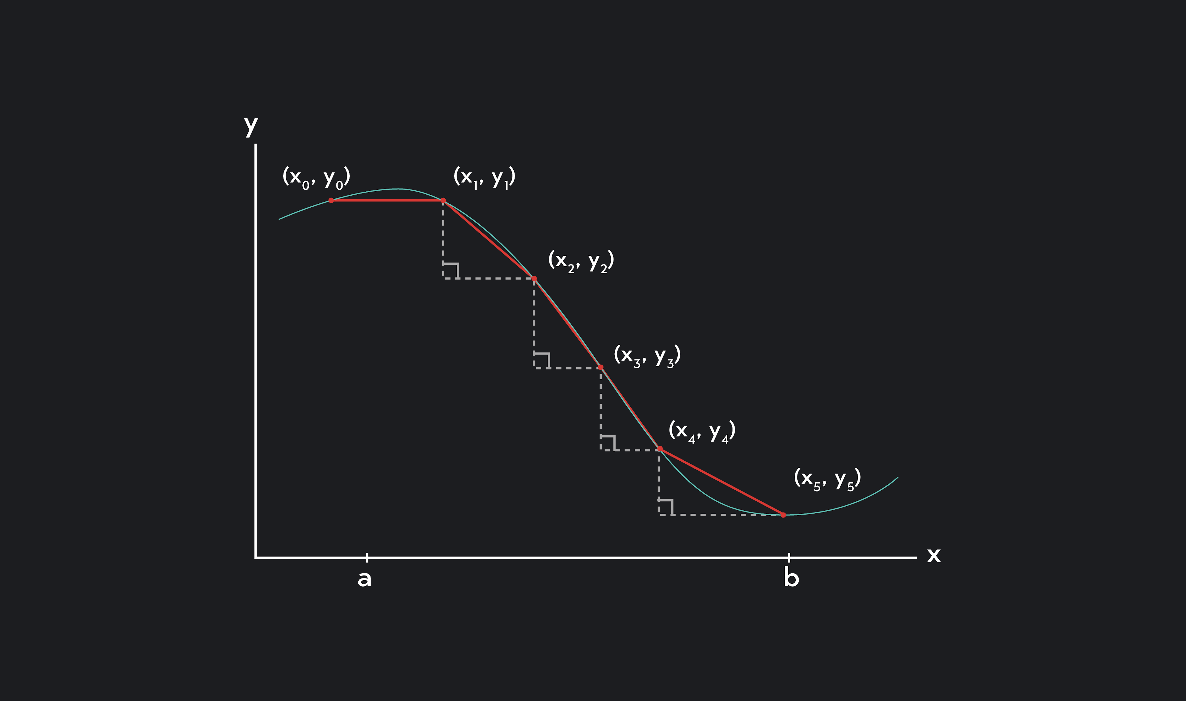
Suppose that $f$ is smooth on $[a, b]$. To approximate the arc length of the curve, we can break the curve into $n$ small sections. Then, we can connect the endpoints of each section with a straight line to form an approximation of the curve.

Using the distance formula, we can determine the length of each straight line segment. Adding up these lengths gives us an approximate answer for the arc length. Below is an example of this process for $n = 5$.

Each straight line segment is the hypotenuse of a right triangle. Then, by the Pythagorean theorem, the length of each straight line segment is given by the formula below. This is called the distance formula.

Because the curve on $[a, b]$ is broken into $n$ pieces using a regular partition over $[a, b]$, we can let the change in horizontal distance be given by $\Delta x$. However, the change in vertical distances varies, so this is given by $\Delta y_i = y_i - y_{i-1}$. Then, we have:

Taking the sum of the lengths of these tiny straight line segments gives us an approximate measurement of the arc length.

Now, notice that $\Delta y_i = y_i - y_{i-1} = f(x_i) - f(x_{i-1})$. This allows us to use the Mean Value Theorem, which states that if $f$ is continuous and differentiable on $[a, b]$, then there exists some point $c$ in $[a, b]$ such that

So, we can say there exists some x_i^*$ in $[x_{i-1}, x_i] such that:

Rearranging this equation, we get:

Substituting in $\Delta y_i = f(x_i) - f(x_{i-1})$ and $\Delta x = x_i - x_{i-1}$, we get:

Using this expression, the arc length can now be approximated as:

Factoring out $\Delta x^2$, we have:

As we break the curve into smaller and smaller sections, the collection of resulting straight line segments begins to match the original curve better and better.

So, as we make $n$ bigger, the curve of $f$ is broken into more and more small pieces, and our approximation of the arc length becomes more and more precise.

Then, by taking the limit of our approximation as $n$ approaches infinity, we can find the precise arc length of $f$ on $[a, b]$.

Note that a definite integral is defined by:

Using this definition, we can say that the arc length is equal to the definite integral below. We have finally derived the arc length equation.

Similarly, if $g(y)$ is a smooth function on $[c, d]$, we can say that

How To Find the Arc Length of a Function

Now that we understand how to derive the arc length integral formula, we can follow the four simple steps below to calculate the arc length of a smooth function on $[a, b]$.

1. Differentiate $f(x)$ to find $f’(x)$.

2. Square $f’(x)$.

3. Plug $[f’(x)]^2$ into the arc length formula and plug $a$ and $b$ into the upper and lower bounds of the integral.

4. Integrate.

How To Find an Arc Length Example

Let’s do one example together to solidify your understanding. Let $f(x) = x^{\frac{3}{2}}$. Find the arc length of $f$ from $x = 4$ to $x = 8$.

1. Differentiating $f(x)$ using the power rule, we have $f’(x) = \frac{3}{2}x^\frac{1}{2}$.

2. Squaring $f’(x)$, we find that $[f’(x)]^2 = {(\frac{3}{2}x^\frac{1}{2})}^2 = \frac{9}{4}x$.

3. Using the arc length formula, our integral is $\int_1^3 \sqrt{1 + \frac{9}{4}x} dx$.

4. We will integrate using u-substitution. (If needed, you can review our guide about what is u-substitution.

Let $u = 1 + \frac{9}{4}x$. Then $du = \frac{9}{4} \, dx$. Then, to keep our equation balanced, we must multiply the integrand by $\frac{4}{9}$. We must also calculate our new bounds in terms of $u$. Plugging $a = 4$ into $u$, we get $u(4) = 10$. Plugging $b = 8$ into $u$, we get $u(8) = 19$. Now, we can integrate. You will need to use your calculator to compute this and get the approximate final answer.

Thus the arc length of $f$ from $x = 4$ to $x = 8$ is approximately 15.1693.

What Is the Surface Area of the Surface of Revolution?

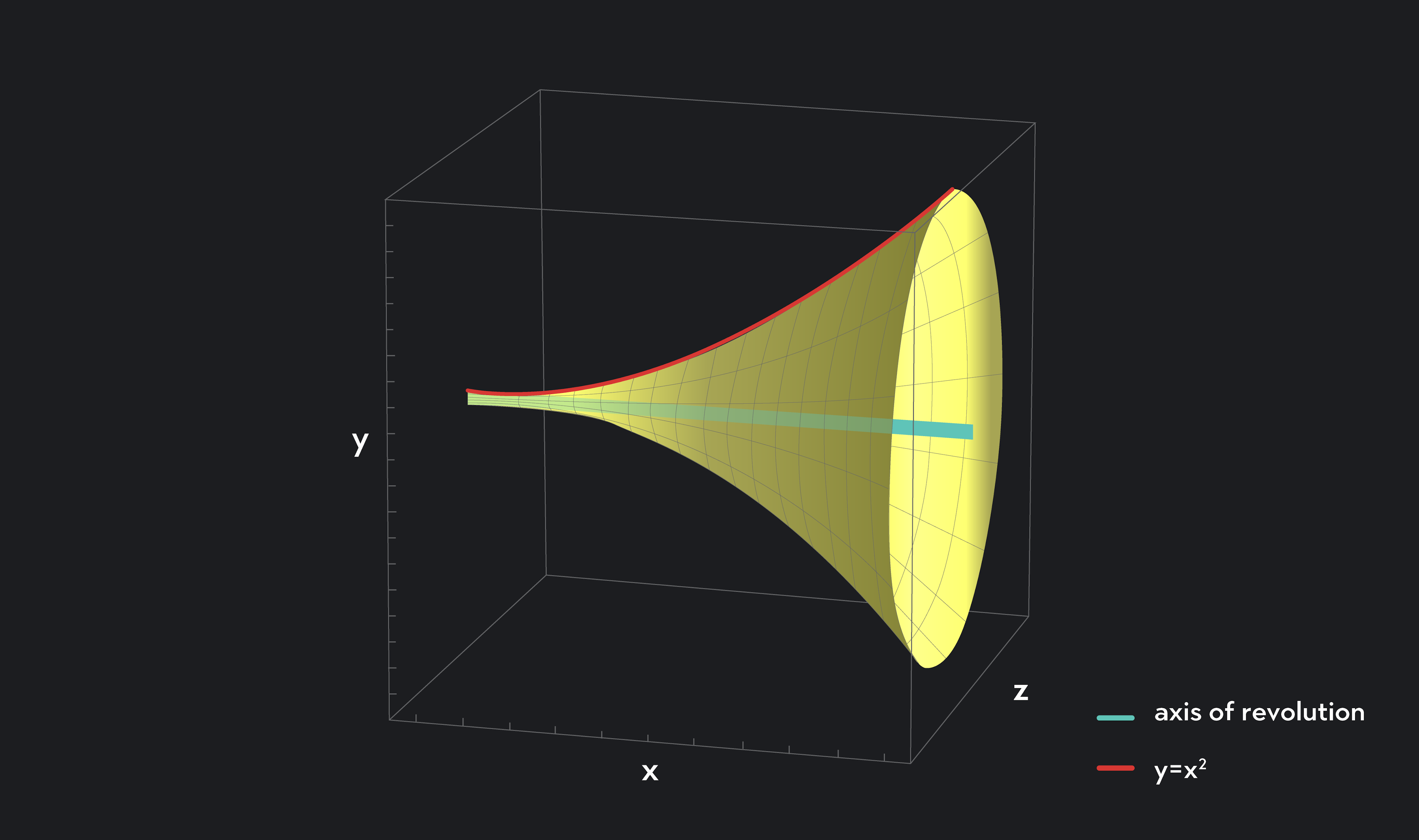
We can create a three dimensional object by rotating the curve of a function 360 degrees about the x-axis. This creates a surface of revolution. For example, the surface of revolution created by revolving $y = x^2$ about the x-axis is given below. Note that our function must be smooth and nonnegative.

Frustum

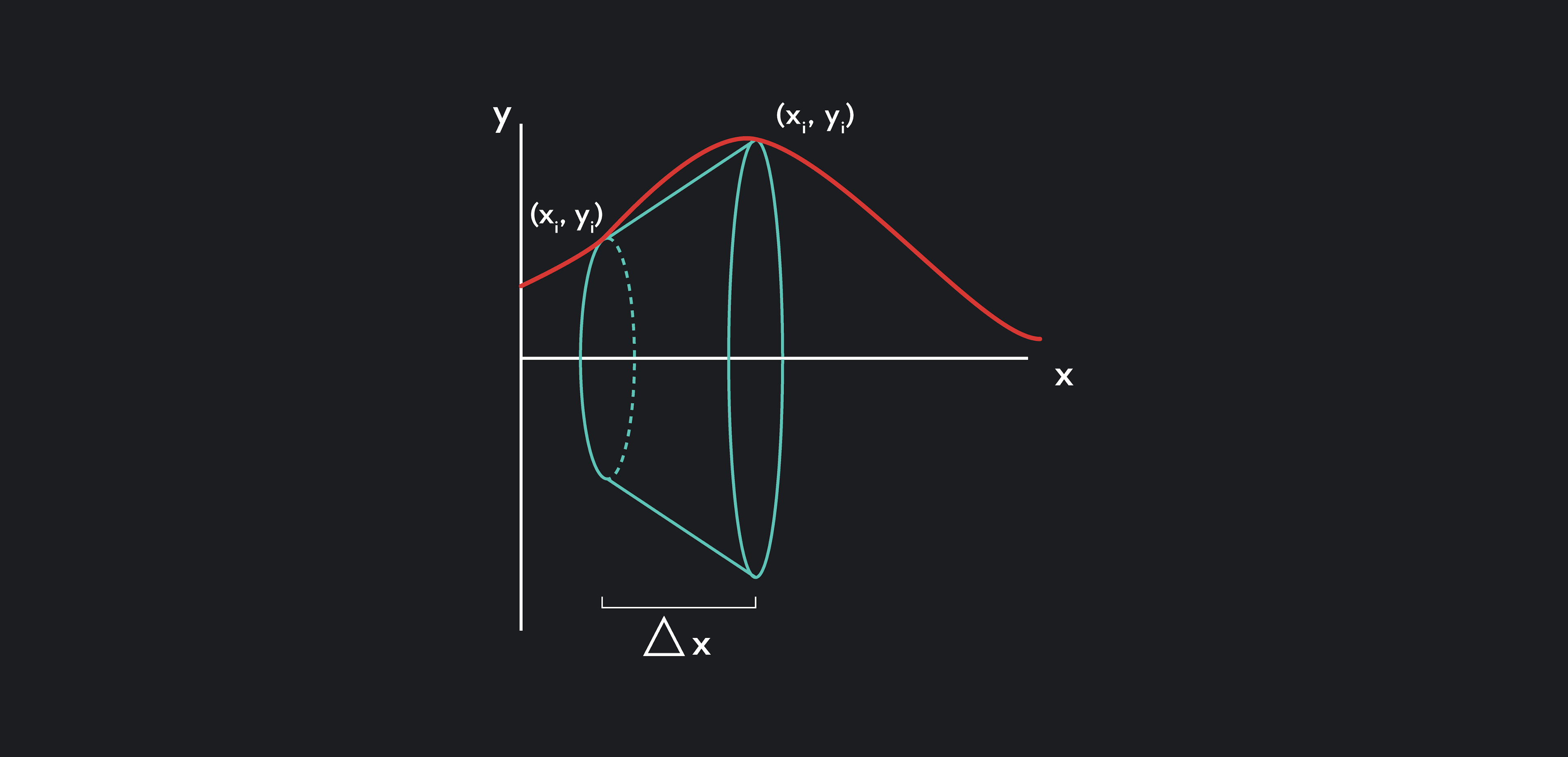
As we did before to derive the arc length formula, imagine breaking the curve of $f$ into $n$ small sections and connecting the endpoints of each section with a straight line segment. Revolving these straight line segments about the x-axis creates a three-dimensional shape that looks like a piece of cone called a frustum. A frustum looks like an ice cream cone with the pointy part removed.

Below is an example of a frustum generated by rotating a straight line segment around the x-axis.

Formula for the Surface Area of a Frustum

So, how do we calculate the surface area of the surface of revolution? Well, we can start by investigating the formula for the surface area of a frustum.

The formula for the lateral surface area of a frustum is given by $SA = 2\pi \frac{(r_1 + r_2)}{2}l$, where $r_1$ and $r_2$ are the radii of the bases and $l$ is the slant height of the frustum.

The radii $r_1$ and $r_2$ are equal to the values $y_i = f(x_i)$ and $y_{i-1} = f(x_{i-1})$, respectively. The slant height $l$ is simply the length of the line segment used to generate the frustum. We already calculated the formula for the length of the straight line segment in our previous work for deriving the arc length formula.

So, we can change the formula for the surface area of a frustum to look like this:

The Intermediate Value Theorem tells us that there exists some value $f(x_i^*)$ between $f(x_{i-1})$ and $f(x_i)$ such that $f(x_i^*) = \frac{f(x_i) + f(x_{i-1})}{2}$, so our equation becomes:

Taking the sum of the surface area of each frustum that is generated by the $n$ straight line segments that approximate the curve of $f$ gives us:

$\text{Surface Area of the Surface of Revolution} \approx \sum_{i = 1}^n 2\pi f(x_i^*) \sqrt{(1 + [f’(x_i^*)]^2)} \Delta x$

Similar to what we determined with the arc length formula, when we break the curve into smaller and smaller sections, the collection of resulting frustums begins to match the surface of revolution better and better.

As we make $n$ bigger, the curve of $f$ is broken into more and more small pieces, and our approximation of the surface area of the surface of revolution becomes more and more precise.

Then, by taking the limit of our surface area approximation as $n$ approaches infinity, we can find the precise surface area of the surface of revolution of $f$ on $[a, b]$.

$\text{SA of the Surface of Revolution} = \lim_{n\to\infty} \sum_{i = 1}^n 2\pi f(x_i^*) \sqrt{(1 + [f’(x_i^*)]^2)} \Delta x$

We can use the definition of a definite integral that was given before to finally determine the formula for the surface area of a surface of revolution given by revolving $f$ around the x-axis on $[a, b]$.

$\text{SA of the Surface of Revolution} = \int_a^b 2\pi f(x) \sqrt{1 + [f’(x)]^2} dx$

Similarly, the surface area of the surface of revolution given by revolving a nonnegative smooth function $g$ around the y-axis on $[c, d]$ is:

$\text{SA of the Surface of Revolution} = \int_c^d 2\pi g(y) \sqrt{1 + [g’(y)]^2} dy$

How To Calculate the Surface Area of a Surface of Revolution

Now that we understand how to derive the formula, we can follow the four simple steps below to calculate the surface area of the surface of revolution of a smooth function on $[a, b]$.

1. Differentiate $f(x)$ to find $f’(x)$.

2. Square $f’(x)$.

3. Plug $[f’(x)]^2$ into the surface area formula and plug $a$ and $b$ into the upper and lower bounds of the integral.

4. Integrate.

Example of How To Find the Surface Area of the Surface of Revolution

We’ll do one simple example together. Let $f(x) = x$. Find the surface area of the surface of revolution on $[0, 1]$ formed by revolving the graph of $f(x)$ around the x-axis.

1. Differentiating $f(x)$ using the power rule, we find the $f’(x) = 1$.

2. Squaring $f’(x)$ gives us 1.

3. Using the surface area formula, our integral is:

4. Integrating gives us:

Thus, the surface area of the surface of revolution of $f(x) = x$ on $[0, 1]$ is $\pi \sqrt{2} \approx 4.4429$.

Explore Outlier's Award-Winning For-Credit Courses

Outlier (from the co-founder of MasterClass) has brought together some of the world's best instructors, game designers, and filmmakers to create the future of online college.

Check out these related courses:

Calculus I

The mathematics of change.

Explore course

Calculus I

The mathematics of change.

Explore course

Intro to Statistics

How data describes our world.

Explore course

Intro to Statistics

How data describes our world.

Explore course

Intro to Microeconomics

Why small choices have big impact.

Explore course

Intro to Microeconomics

Why small choices have big impact.

Explore course